Download
1 / 23
230 likes | 318 Vues
Explore the objectives and methodologies of single variable between-subjects research, including the general linear model, ANOVA, effect sizes, and controlling variables for cause and effect studies.

E N D
Slides to accompany Weathington, Cunningham & Pittenger (2010), Chapter 12: Single Variable Between-Subjects Research
Objectives • Independent Variable • Cause and Effect • Gaining Control Over the Variables • The General Linear Model • Components of Variance • The F-ratio • ANOVA Summary Table • Interpreting the F-ratio • Effect Size and Power • Multiple Comparisons of the Means
Multi-level Independent Variable • More than 2 levels of the IV • Permits more detailed analysis • Can’t identify certain types of relationships with only two data points (Figure 12.1) • Can increase a study’s power by reducing variability within the multiple treatment condition groups
Searching for Cause and Effect • Identifying differences among multiple groups is a starting point for causal study • Control is the key: • Through research design • Through research procedure
Control through Design • Most easily secured in a true experiment • You manipulate and control the IV • Control groups are possible isolating effects of IV • You control random assignment of participants • Helps to reduce confounding effects
Control through Procedure • Each participant needs to experience the same process (except the manipulation) • Systematic • Identifying and trying to limit as many confounding factors as possible • Pilot studies are a great way to test your process and your control strategies
General Linear Model • Xij = µ + αj + εij • A person’s performance (score = Xij) will reflect: • Typical score in that group (µ) • Effect of the treatment/manipulation (αj) • Random error (εij) • Ho: all µi equal
GLM and Between-Subj. Research • Goal is to determine proportion of total variance due to IV and proportion due to random error • Size of between-groups variance is due to error (εij) and IV (αj) • If b-g variance > w-g variance IV has some effect
ANOVA • Compares different types of variance • Total variance = variability among all participants’ scores (groups do not matter) • Within-groups variance = average variability among scores within a group or condition (random) • Between-groups variance = variability among means of the different treatment groups • Reflects joint effects of IV and error
F-ratio • Allows us to determine if b-g variance > w-g variance • F = Treatment Variance + Error Variance Error Variance • F = MSbetween/MSwithin
F-ratio: No Effect • Treatment group M may not all be exactly equal, but if they do not differ substantially relative to the variability within each group nonsignificant result • When b-g variance = w-g variance, F = 1.00, n.s.
F-ratio: Significant Effect • If IV influences DV, then b-g variance > w-g variance and F > 1.00 • Examining the M can highlight the difference(s)
F-ratio Distribution • Represents probability of various F-ratios when Ho is true • Shape is determined by two df • 1st = b-g = (# of groups) - 1 • 2nd = w-g = (# of participants in a group) – 1 • Positive skew, αon right extreme region
Summarizing ANOVA Results • Figure 12.7 • Using the critical value from appropriate table in Appendix B, if Fobs > Fcrit significant difference among the M • Rejecting Ho requires further interpretation • Follow-up contrasts
Interpreting F-ratio • Omega squared indicates degree of association between IV and DV • f is similar to d for the t-test • Typically requires further M comparisons • t-test time, but with reduced α to limit chances of committing a Type I error
Multiple Means Comparisons • You could consider lowering α to .01, but this would increase your Type II probability • Instead use a post-hoc correction for α: • αe= 1 – (1 – αp)c • Tukey’s HSD = difference required to consider M statistically different from each other
What is Next? • **instructor to provide details