Simple Linear Regression in Engineering and Science
Learn to build empirical models, estimate parameters using least squares, analyze residuals, make predictions, apply correlation, and execute hypothesis tests effectively.

Simple Linear Regression in Engineering and Science
E N D
Presentation Transcript
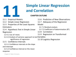
11 Simple Linear Regression and Correlation CHAPTER OUTLINE 11-1 Empirical Models 11-2 Simple Linear Regression 11-3 Properties of the Least Squares Estimators 11-4 Hypothesis Test in Simple Linear Regression 11-4.1 Use of t-tests 11-4.2 Analysis of variance approach to test significance of regression 11-5 Confidence Intervals 11-5.1 Confidence intervals on the slope and intercept 11-5.2 Confidence interval on the mean response 11-6 Prediction of New Observations 11-7 Adequacy of the Regression Model 11-7.1 Residual analysis 11-7.2 Coefficient of determination (R2) 11-8 Correlation 11-9 Regression on Transformed Variables 11-10 Logistics Regression Chapter 11 Table of Contents
Learning Objectives for Chapter 11 After careful study of this chapter, you should be able to do the following: • Use simple linear regression for building empirical models to engineering and scientific data. • Understand how the method of least squares is used to estimate the parameters in a linear regression model. • Analyze residuals to determine if the regression model is an adequate fit to the data or to see if any underlying assumptions are violated. • Test the statistical hypotheses and construct confidence intervals on the regression model parameters. • Use the regression model to make a prediction of a future observation and construct an appropriate prediction interval on the future observation. • Apply the correlation model. • Use simple transformations to achieve a linear regression model. Chapter 11 Learning Objectives
11-1: Empirical Models • Many problems in engineering and science involve exploring the relationships between two or more variables. • Regression analysisis a statistical technique that is very useful for these types of problems. • For example, in a chemical process, suppose that the yield of the product is related to the process-operating temperature. • Regression analysis can be used to build a model to predict yield at a given temperature level.
11-1: Empirical Models Figure 11-1Scatter Diagram of oxygen purity versus hydrocarbon level from Table 11-1.
11-1: Empirical Models Based on the scatter diagram, it is probably reasonable to assume that the mean of the random variable Y is related to x by the following straight-line relationship: where the slope and intercept of the line are called regression coefficients. The simple linear regression model is given by where is the random error term.
11-1: Empirical Models We think of the regression model as an empirical model. Suppose that the mean and variance of are 0 and 2, respectively, then The variance of Y given x is
11-1: Empirical Models • The true regression model is a line of mean values: • where 1 can be interpreted as the change in the mean of Y for a unit change in x. • Also, the variability of Y at a particular value of x is determined by the error variance, 2. • This implies there is a distribution of Y-values at each x and that the variance of this distribution is the same at each x.
11-1: Empirical Models Figure 11-2The distribution of Y for a given value of x for the oxygen purity-hydrocarbon data.
11-2: Simple Linear Regression • The case of simple linear regression considers a single regressoror predictorx and a dependent or response variableY. • The expected value of Y at each level of x is a random variable: • We assume that each observation, Y, can be described by the model
11-2: Simple Linear Regression • Suppose that we have n pairs of observations (x1, y1), (x2, y2), …, (xn, yn). Figure 11-3Deviations of the data from the estimated regression model.
11-2: Simple Linear Regression • The method of least squares is used to estimate the parameters, 0 and 1 by minimizing the sum of the squares of the vertical deviations in Figure 11-3. Figure 11-3Deviations of the data from the estimated regression model.
11-2: Simple Linear Regression • Using Equation 11-2, the n observations in the sample can be expressed as • The sum of the squares of the deviations of the observations from the true regression line is
11-2: Simple Linear Regression Definition
11-2: Simple Linear Regression Notation
11-2: Simple Linear Regression Example 11-1
11-2: Simple Linear Regression Example 11-1
11-2: Simple Linear Regression Example 11-1 Figure 11-4Scatter plot of oxygen purity y versus hydrocarbon level x and regression model ŷ = 74.20 + 14.97x.
11-2: Simple Linear Regression Example 11-1
11-2: Simple Linear Regression Estimating 2 The error sum of squares is It can be shown that the expected value of the error sum of squares is E(SSE) = (n – 2)2.
11-2: Simple Linear Regression Estimating 2 An unbiased estimator of 2 is where SSE can be easily computed using
11-3: Properties of the Least Squares Estimators • Slope Properties • Intercept Properties
11-4: Hypothesis Tests in Simple Linear Regression 11-4.1 Use of t-Tests Suppose we wish to test An appropriate test statistic would be
11-4: Hypothesis Tests in Simple Linear Regression 11-4.1 Use of t-Tests The test statistic could also be written as: We would reject the null hypothesis if
11-4: Hypothesis Tests in Simple Linear Regression 11-4.1 Use of t-Tests Suppose we wish to test An appropriate test statistic would be
11-4: Hypothesis Tests in Simple Linear Regression 11-4.1 Use of t-Tests We would reject the null hypothesis if
11-4: Hypothesis Tests in Simple Linear Regression 11-4.1 Use of t-Tests An important special case of the hypotheses of Equation 11-18 is These hypotheses relate to the significance of regression. Failure to reject H0 is equivalent to concluding that there is no linear relationship between x and Y.
11-4: Hypothesis Tests in Simple Linear Regression Figure 11-5The hypothesis H0: 1 = 0 is not rejected.
11-4: Hypothesis Tests in Simple Linear Regression Figure 11-6The hypothesis H0: 1 = 0 is rejected.
11-4: Hypothesis Tests in Simple Linear Regression Example 11-2
11-4: Hypothesis Tests in Simple Linear Regression 11-4.2 Analysis of Variance Approach to Test Significance of Regression The analysis of variance identity is Symbolically,
11-4: Hypothesis Tests in Simple Linear Regression 11-4.2 Analysis of Variance Approach to Test Significance of Regression If the null hypothesis, H0: 1 = 0 is true, the statistic follows the F1,n-2 distribution and we would reject if f0 > f,1,n-2.
11-4: Hypothesis Tests in Simple Linear Regression 11-4.2 Analysis of Variance Approach to Test Significance of Regression The quantities, MSR and MSE are called mean squares. Analysis of variance table:
11-4: Hypothesis Tests in Simple Linear Regression Example 11-3
11-5: Confidence Intervals 11-5.1 Confidence Intervals on the Slope and Intercept Definition
11-5: Confidence Intervals Example 11-4
11-5: Confidence Intervals 11-5.2 Confidence Interval on the Mean Response Definition
11-5: Confidence Intervals Example 11-5
11-5: Confidence Intervals Example 11-5
11-5: Confidence Intervals Example 11-5
11-5: Confidence Intervals Figure 11-7 Figure 11-7Scatter diagram of oxygen purity data from Example 11-1 with fitted regression line and 95 percent confidence limits on Y|x0.
11-6: Prediction of New Observations If x0 is the value of the regressor variable of interest, is the point estimator of the new or future value of the response, Y0.
11-6: Prediction of New Observations Definition
11-6: Prediction of New Observations Example 11-6
11-6: Prediction of New Observations Example 11-6