The Quality Improvement Model
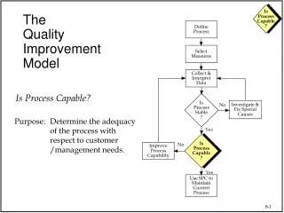
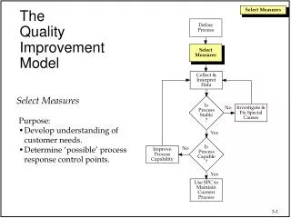
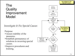
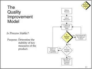
The Quality Improvement Model. Define Process. Select Measures. Collect & Interpret Data. Is Process Stable?. Is Process Stable ?. No. Investigate & Fix Special Causes. Purpose: Determine the stability of key measures of the product. Yes. Is Process Capable ?. No.

The Quality Improvement Model
E N D
Presentation Transcript
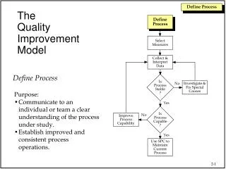
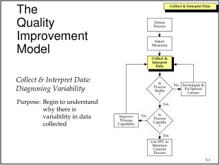
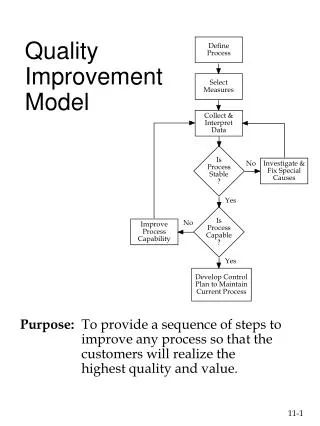
TheQualityImprovementModel Define Process Select Measures Collect & Interpret Data Is Process Stable? IsProcessStable? No Investigate & Fix Special Causes Purpose: Determine the stability of key measures of the product. Yes IsProcessCapable? No Improve Process Capability Yes Use SPC to Maintain Current Process
Types of VariationCommon Causes Causes that are inherent in the process over time, and affect all outcomes of the process. • Ever-present • Create small, random fluctuations in the process • Lots of them • The sum of their effects creates the expected variability • Predictable Run Chart Quality Characteristic Time
Types of VariationSpecial Causes • Causes that are not present in the • process all the time, but arise • because of specific circumstances. • Not always present in the process • Can create large process disturbances, or sustained shifts • Relatively few in number • Pull the process beyond the expected level of variability • Unpredictable Run Chart Quality Characteristic Time Control charts help identify the presence of special causes.
Control Chart UCL CL LCL 2 4 6 8 10 12 14 16 18 20 22 24 26 28 30 32 Run Order Control Chart Components • Run chart of the data • Center Line (CL) • A line at the average of the data or target of the process • Upper Control Limit (UCL) • A line at the upper limit of expected variability • Lower Control Limit (LCL) • A line at the lower limit of expected variability The control limits are based on data collected from the process.
Rules for Separating Common & Special Causes Two commonly used signals of special causes are: Rule 1: Any point above the Upper Control Limit (UCL) or below the Lower Control Limit (LCL) Rule 2: 8 points in a row on the same side of the center line (CL) Note: Additional rules do exist.
Evaluation of Individuals Data s c R , n = 2 s • s • • s • c • • • • • • • • • • • • • • • • • • • • • • • • • • • • • • • T X • Target • • • • • • • • • • • • • • • • • • • • • • • Order of Production s Measures Variation in All Data s Used to Estimate 'Spread' Does Not Reflect 'Capability' Should Not Be Used for Calculating Control Chart Limits s Measures Variation in Successive Values c Used to Estimate the Potential Capability Should Be Used to Calculate Trial Control Chart Limits
Estimating Sigma (Standard Deviation) 2 n X – X å i Total s s s s i = 1 = n – 1 n X – X å i i – 1 R Short-Term s i = 2 s = = c c 1.128 n – 1 1.128 In existing data, Sigma C is a better estimate of the common cause variability… Since it eliminates variation due to cycles, shifts, etc…(Special Causes). Therefore, Sigma C (from edited moving ranges) is always used to calculate control limits!
Problem: Individuals Chart Calculations 93.2 5 3.9 2 89.3 4 7.3 2 3 96.6 16.7 2 79.9 2 y 7.8 Problem #13 l 2 i a 87.7 D 1 1.1 2 = y 88.8 0 0.1 c 2 n e 88.7 u 9 3.1 1 q e r 85.6 8 F 4.0 1 81.6 7 12.6 1 94.2 6 3.2 1 97.4 5 4.5 1 92.9 4 6.3 1 86.6 3 2.9 1 2 89.5 5.3 1 Line 1 - First 25 Points Only 84.2 1 6.8 1 91.0 0 3.4 1 94.4 9 0.4 94.0 8 3.1 90.9 7 1.8 89.1 6 7.5 81.6 5 10.0 91.6 4 2.4 94.0 3 2.8 R O 91.2 2 F 3.6 T 87.6 - 1 R A H ) C R ) M R L X ( ( O e M t g n R 1 n e & a e T m n r R e i o N X L r t g u a n O r s R i e e v e a t C m p M a e o X i O D M M T
Individuals Chart Calculations L i n e 1 - F i r s t 2 5 P o i n t s O n l y C o n t r o l C h a r t f o r _ _ _ _ _ _ _ _ _ _ _ _ _ _ _ _ _ _ _ _ _ _ _ _ _ _ _ _ _ _ _ X & M R C H A R T S - C a l c u l a t i o n W o r k s h e e t M R = C u r r e n t M e a s u r e m e n t – P r e v i o u s M e a s u r e m e n t T o t a l o f M R s R = = = T o t a l n u m b e r M R s T o t a l o f M e a s u r e m e n t s X = = = T o t a l n u m b e r o f M e a s u r e m e n t s ´ U C L R = 3 . 2 6 7 L C L = 0 M R M R ´ = 3 . 2 6 7 = s R = = = c 1 . 1 2 8 1 . 1 2 8 s s L C L = X – 3 U C L = X + 3 c X c X U C L = + 3 ( ) L C L = – 3 ( ) X X U C L = + L C L = – X X U C L = L C L = X X
Minitab: Creating Individuals Control Charts • Open Minitab Software and the Line 1.MTW Worksheet. • Create an Individuals Control Chart following the commands in the notes. • Your output should look like the charts below:
Minitab: Creating Individuals Control Charts • Open Problem 14.MTW located in the Minitab Datasets folder. • Use Minitab to create an Individuals and Moving Range control chart for X in column C1. • What do you notice about the X and MR Charts? • What should you do to establish control limits?
Minitab: Creating Individuals Control Charts With Range Edited Limits • As you noticed the moving range control chart for problem 14 has two ranges that are above the upper control limit. • So, a special cause source of variation is included in the limits calculation. • The special cause needs to be removed and the limits re-calculated. • Row 24 is the data point causing the moving ranges to be out of the limits. • Use the brush tool to select and update the control chart or create a new column without data point #24 (Remember to use the Backspace). • These were taught in the Introduction to Minitab Course which is a pre-requisite for the SPC course. • Brush tool – Page 13 Introduction to Minitab book
Minitab: Creating Individuals Control Charts With Range Edited Limits • The chart below shows the updated control charts without point #24. • The updated moving range chart shows more moving ranges outside of limits. • These are caused by rows 7 and 29. • Remove the data points and update the control charts again.
Minitab: Creating Individuals Control Charts With Range Edited Limits • The second updated Moving Range chart does not have any points outside of limits • The objective is to calculate control limits that represent common cause sources of variation only. • However, stop editing data points once 10 to 20% of the data has been edited. • If the initial data has this many special causes, the limits will identify plenty special causes in the future for you to work on.
Minitab: Obtain Statistics to Calculate Limits for Continuous Process Monitoring Select I-MR Options in the I-MR dialog box Choose Storage and select Means and Standard deviations
Minitab: Obtain Statistics to Calculate Control Limits Continued Two new columns are created Mean1 – Average of your data STDE1 – Sigma_C
Process Stability Stable Process A process in which the key measures of the output from the process show no signs of special causes. Variation is a result of common causes only. Unstable Process A process in which the key measures of the output from the process show signs of special causes in addition to common causes. Variation is a result of both common and special causes.
A Stable Process U C L • • • • • • • • • • • • • • • • • • • • • • • • • • • • • • • • • • • • • • • • • • • • • • • • • • • • • • • • • • • • • • • • • • • • • • • • • • • • • • • • L C L C o m m o n C a u s e s A l o n e A r e A t W o r k : • B e h a v e s i n a R a n d o m M a n n e r • N o C y c l e s • N o R u n s • N o T r e n d s • N o S h i f t s • N o D e f i n e d P a t t e r n s
A Stable Process: Sigma S = Sigma C L o w e r U p p e r S p e c S p e c C e n t e r i n g O . K . C a p a b i l i t y A d e q u a t e N o A c t i o n N e e d e d s s X 3 3 c c C A P A B I L I T Y S P R E A D L o w e r U p p e r S p e c S p e c C e n t e r i n g O f f C a p a b i l i t y A d e q u a t e S h i f t C e n t e r i n g B y A l t e r i n g A i m o f P r o c e s s L o w e r U p p e r S p e c S p e c C e n t e r i n g O . K . C a p a b i l i t y I n a d e q u a t e C h a n g e P r o c e s s
Un-Stable Process • • • • U C L • • • • • • • • • • • • • • • • • • • • • • • • • • • • • • • • • • • • • • • • • • • • • • • • • • • • • • • • • • • • • • • • • • • • • • • • • • • • • L C L A s s i g n a b l e C a u s e ( s ) A r e P r e s e n t I n A d d i t i o n T o C o m m o n C a u s e V a r i a t i o n L o o k F o r : • P o i n t s O u t s i d e t h e C o n t r o l L i m i t s • S h i f t s • C y c l e s • R u n s • T r e n d s
Un-Stable Process: Sigma S Not Equal to Sigma C L o w e r U p p e r S p e c S p e c S p r e a d W i t h i n S p e c i f i c a t i o n s D e t e r m i n e C a u s e o f I n s t a b i l i t y a n d C o r r e c t I f E c o n o m i c a l l y F e a s i b l e C A P A B I L I T Y S P R E A D L o w e r U p p e r S p e c S p e c S p r e a d O u t s i d e S p e c i f i c a t i o n s C a p a b i l i t y A d e q u a t e D e t e r m i n e C a u s e o f d C o r r e c t I n s t a b i l i t y a n L o w e r U p p e r S p r e a d O u t s i d e S p e c S p e c S p e c i f i c a t i o n s C a p a b i l i t y I n a d e q u a t e C h a n g e P r o c e s s - A t t e m p t t o A c h i e v e A t L e a s t P a r t i a l I m p r o v e m e n t
Control Chart 5 b* Histogram 4 LS US 3 UCL=2.2 2 Avg=1.4 1 LCL=0.5 0 0 1 2 3 4 5 20 40 60 80 100 120 140 Sample b* Polymer Manufacturing Data Note: b* is a measure of yellowness Histogram does not show whether the process is stable!
What’s Wrong With Putting SpecificationLimits on Control Charts? Case 1: (Specifications wider than Control Limits) USL x UCL x x CL x x LCL x LSL x Case 2: (Control Limits wider than Specifications) UCL x USL x x CL x x LSL x LCL In both cases, specification limits on control charts cause you to take the wrong action.
Histograms & Control Charts • Control Charts • Real-time evaluation • Help identify presence of special causes • Assess past and present stability of process Histograms • Plot past data • Cannot tell if process is stable • Only useful for prediction if the process is stable
20 18 16 14 12 10 8 6 4 2 0 IsProcessStable? Pump Maintenance Data Number of Failures UCL=11.4 Avg=4.8 LCL=None 2 4 6 8 10 12 14 16 18 20 22 24 Week Are there any signals of special causes? Circle them.
55 UCL=51.6 Time (Minutes) 50 Avg=45.9 45 LCL=40.2 40 35 5 10 15 20 25 30 35 Day Driving to Work Data The next 5 observations are: 47, 46, 43, 52, 45. Plot them. Are there any signals of special causes? Circle them.
14 13 12 11 Time (Days) 10 UCL=9.5 9 8 7 6 Avg=5.0 5 4 3 2 1 LCL=0.5 0 2 4 6 8 10 12 14 16 18 20 Week Sample Taken Purchase Order Data Are there any signals of special causes? Circle them.
0.30 0.25 UCL 0.20 0.15 Avg=0.123 0.10 0.05 LCL 0.00 2 4 6 8 10 12 14 16 18 20 22 24 26 28 30 Shipping Data p (fraction nonconforming) Week Are there any signals of special causes? Circle them.
Instrument Measures x (X-bar) charts Individuals (x) charts Range (R) charts Moving Range (MR) charts Arithmetic Moving Average charts Exponentially Weighted Moving Average charts Cusum charts Quality ImprovementTypes of Control Charts • Counting Measures • p charts • np charts • c charts • u charts “When you have a problem to solve, you want to choose the right tool.”
• • • % of Customers Ranking Eastman as #1 Supplier • • • • • • • • • • • • • • • • • • • • • • • • • • • • • • Time ExercisesCircle any signals of special causes you find in the following control charts. Example 1 Example 2 Monthly Sales Time
• • • • • • % Defective • • • • • • • • • • • • • • • • • • • • • • • • • Time Skill Check - Continued Example 3 Example 4 • Number of Lost-Time Accidents • Time
Exercises 1.) Your Catapult Team should complete page 9 of the “Catapult Process” handout. 2.) Be ready to present your results in PowerPoint Limit yourselves to 10 minutes for this exercise.