Download
1 / 86
910 likes | 1.03k Vues
Explore laminar and turbulent flows, stability mechanisms, and transition to turbulence in aerodynamics. Learn theory and computation with suggested literature and video resources.

E N D
AA-277Instability and transition to turbulence André V. G. Cavalieri Peter Jordan (Visiting researcher, Ciência Sem Fronteiras)
Laminar flows Lower skin friction and heat transfer Prone to flow separation Steady flows, no noise generation Turbulent flows Increased skin friction and heat transfer Turbulent mixing Less prone to separation Aerodynamic noise Instability and transition to turbulence instability Challenges: 1 – Predict transition to turbulence 2 – Understand mechanisms of transition 3 – Flow control: delay, or simply avoid turbulence
Instability and transition to turbulence • Are there steady (laminar) solutions to the Navier-Stokes equations? • Yes! • Example: zero-pressure-gradient boundary layer (Blasius): solution for arbitrary Re • Are there small (or sometimes not so small) disturbances in the environment? • Yes! • Surface roughness • Vibration • Sound waves • Incoming vorticity • A mosquito flying nearby • Are the steady solutions stable to these disturbances? • Answer: it depends... strongly on Re (but also on M) • Unstable laminar solutions will not prevail on nature
This course • Theory • Suggested literature: • Criminale, Jackson & Joslin, Theory and computation of hydrodynamic stability, Cambridge University Press, 2003 • Schmid & Henningson, Stability and transition in shear flows, Springer, 2001 • + various articles to be provided during the course • Computation • Matlab programming • Trefethen, Spectral methods in Matlab • Boyd, Chebyshev and Fourier spectral methods • Lectures with assignments • Goals: • Build a toolbox to solve some canonical stability problems • Learn with examples • Grades: • Theoretical and computational assignments • Material can be found in ftp://161.24.15.247/Andre/AA277
Videos! Rayleigh-Taylor instability http://www.youtube.com/watch?v=NI85oC-3mJ0 Pipe flow: Reynolds experiment (1883) http://www.youtube.com/watch?v=xiX5PfFxmIs Boundary-layer transition: Tollmien-Schlichting waves http://www.youtube.com/watch?v=nb22g6ky2XE Kelvin-Helmholtz instability http://www.youtube.com/watch?v=UbAfvcaYr00 Rayleigh-Bénard convection http://www.youtube.com/watch?v=UhImCA5DsQ0
Videos! Rayleigh-Taylor instability http://www.youtube.com/watch?v=NI85oC-3mJ0 Pipe flow: Reynolds experiment (1883) http://www.youtube.com/watch?v=xiX5PfFxmIs Boundary-layer transition: Tollmien-Schlichting waves WAVES!!! http://www.youtube.com/watch?v=nb22g6ky2XE Kelvin-Helmholtz instability http://www.youtube.com/watch?v=UbAfvcaYr00 Fourier Rayleigh-Bénard convection http://www.youtube.com/watch?v=UhImCA5DsQ0
Basic equations: Rayleigh and Orr-Sommerfeld equations Basic equations for two-dimensional incompressible flow with constant viscosity Mass conservation Navier-Stoles equation
Basic equations: Rayleigh and Orr-Sommerfeld equations Mass conservation, non-dimensional Navier-Stoles equation, non-dimensional
Basic equations: Rayleigh and Orr-Sommerfeld equations << We consider infinitesimal disturbances to the base flow, such that << Linearisation is formally justified (but only for initial stages of transition) Tools for linear PDEs: Superposition of solutions Fourier transforms Linear algebra Linear is simpler!
Basic equations: Rayleigh and Orr-Sommerfeld equations tedious but straightforward algebra
Basic equations: Rayleigh and Orr-Sommerfeld equations Other variables:
Basic equations: Rayleigh and Orr-Sommerfeld equations • Coefficients are • constant in x and t • variable in y Normal mode Ansatz: • Wave propagating in x, with: • phase velocity c • wavenumber α • frequency ω=αc • All complex-valued!
Basic equations: Rayleigh and Orr-Sommerfeld equations • Coefficients are • constant in x and t • variable in y Normal mode Ansatz:
Basic equations: Rayleigh and Orr-Sommerfeld equations • Coefficients are • constant in x and t • variable in y Normal mode Ansatz: Neglect viscous effects:
Basic equations: Rayleigh and Orr-Sommerfeld equations Normal mode Ansatz: 4th order, 4 BCs 2nd order, 2 BCs Boundary conditions: Rigid wall: v = 0 (normal velocity is zero) – Rayleigh & Orr-Sommerfeld dv/dy = 0 (since u=0 and du/dx=0, no-slip condition) – only O-S Infinity: bounded v,dv/dy
Basic equations: Rayleigh and Orr-Sommerfeld equations Normal mode Ansatz: • Temporal stability: • wavenumber α is real-valued • frequency ω= ωR + ωI (=αc) is complex-valued • Space-periodic disturbances are added to the base-flow • Will they grow or decay in time?
Basic equations: Rayleigh and Orr-Sommerfeld equations Normal mode Ansatz: • Spatial stability: • frequency ω is real-valued • wavenumber α=αR+iαI is complex-valued • Time-periodic disturbances are added to the base-flow • Will they grow or decay in space? • (see Matlab demo)
Temporal stability Real-valued wavenumber is given Base-flow U is given Reynolds number is given c and v are unknowns Rearrange O-S equation as or
Temporal stability Rearrange O-S equation as or or Generalised eigenvalue problem with linear operators L and F c is the eigenvalue Numerics: discretise operators as matrices, then eig(L,F)
A simpler eigenvalue problem or Let’s first look at a simpler eigenvalue problem • with BC: v=0 for y=-1 and y=1 • This problem appears in: • Linear acoustics • Vibration of membranes • Heat transfer • etc
A simpler eigenvalue problem or Let’s first look at a simpler eigenvalue problem with BC: v=0 for y=-1 and y=1 Analytical solution:
A simpler eigenvalue problem Let’s first look at a simpler eigenvalue problem with BC: v=0 for y=-1 and y=1 Analytical solution: • Numerical solution: needs discretisation of derivative in matrix form • i.e. a differentiation matrix • Choices to build differentiation matrices: • Finite differences (exemple: EVPExample_FiniteDifferences.m) • Spectral method (exemple: EVPExample_Chebyshev.m)
Finite differences v is sampled at N gridpoints, spacing=Δx interior points: centered differences boundary: forward or backward differences (less accurate) Derivative is estimated from values of function on the neighbourhood of xi Differentiation matrix is sparse Freedom to choose the grid
Pseudo-spectral method – Chebyshev polynomials Tn(x) Orthogonal basis in [-1,1] Functions in [-1,1] can be expanded in Chebyshev polynomials Derivatives:
Pseudo-spectral method v is sampled at N+1 Chebyshev gridponts (clustered near boundaries) • Find the coefficients of N+1 Chebyshev polynomials from N+1 values of v • Calculate derivatives of Chebyshev polynomials • Calculate values of dv/dy at the gridpoints • Gather everything inside a single matrix Trefethen 2001 Derivative is estimated from polynomial fit applied to N+1 samples Differentiation matrix is full Grid must be of Chebyshev points See chebyshev_introduction.m
Finite differences x pseudo-spectral method Error in the calculation of the derivative Finite differences: algebraic convergence Spectral: exponential convergence machine precision
Finite differences x pseudo-spectral method 2nd-order finite differences Pseudo-spectral 0.01 error • Some eigenvalues (and eigenfunctions) well converged, • but some (at least half) should not be trusted! • Pseudo-spectral method better suited for accurate predictions • But: revival of finite differences due to sparse-matrix algorithms • (compensate with higher N) – see Gennaro et al. 2013
Exercise – numerical solution of Rayleigh equation (temporal stability) Rayleigh equation, rearranged for temporal stability or Exercise: #1: Adapt the code to solve to solve the temporal stability problem for the Rayleigh equation for a mixing layer (U=0.5(1+tanh(y))), with BC: v 0 for y ±∞ (numerically: v=0 for y= ±H, H>>1) Start with α=0.1. Compare with Michalke (1964).
Exercise – numerical solution of Rayleigh equation (temporal stability) Useful Matlab commands (help can be obtained with comands “help” and “doc”): diag(U): diagonal matrix, main diagonal = vector U II = eye(size(D)): identity matrix, same size as matrix D ZZ = zeros(size(D)): matrix of zeros, same size as matrix D H = 20;y = y*H; D = D/H; D2 = D2/(H^2); : stretches domain from [-1:1] to [-H:H] A*B is the standard matrix multiplication (number of lines of A should be equal to number of columns of B) A.*B is an element-to-element multiplication (dimensions of A and B shoud be equal) A^2 is A*A (A should be a square matrix) A.^2 is A.*A (A can have any size; could be a vector) A(1,:) means all elements in line 1 of matrix A A(:,5) means all elements in column 5 of matrix A
Expected results Kelvin-Helmholtz (K-H) mode Conjugate of K-H
Expected results If the c, v pair is a solution (eigenvalue-eigenfuncion) of the Rayleigh equation the c*, v* pair is also a solution. Is this true for the Orr-Sommerfeld equation?
Expected results, α=0.1, absolute value of eigenfunction exponential decay exponential decay Kelvin-Helmholtz (K-H) mode artificial boundary condition (v=0)
Expected results, α=0.1 In the region where U is constant, Rayleigh equation reduces to If c≠ U then Plus or minus signs are chosen such that solution be bounded at infinity.
Expected results, absolute value of eigenfunction α=0.1 α=0.4 Artificial boundary condition is more problematic at low α. • Domain size should be large compared to the wavelength
Expected results, absolute value of eigenfunction α=0.1 α=0.4 Solution: mapping from infinite (z) to finite domain (y) See appendix E of Boyd for expressions of derivatives
Expected results Kelvin-Helmholtz (K-H) mode Temporal growth rate: ωi=αci What is the fastest growing wavenumber? What is the wavelength of fastest growing disturbances?
Expected results Temporal growth rate of Kelvin-Helmholtz mode • This result shows: • Wavenumber of most amplified disturbances • Growth rate of each amplified wavenumber • Range of amplified wavenumbers
Expected results What is the “preferred” wavelength?
Expected results Kelvin-Helmholtz (K-H) mode Phase speed of disturbances: cr What is the phase speed (convection velocity) of the amplified disturbances?
Expected results Phase speed of Kelvin-Helmholtz mode • For temporal stability, phase speed = ½ • Average speed between two streams • What happens for U(y)=tanh(y)?
Expected results Michalke 1964, U = ½(1+tanh(y)) U = tanh(y) Result: cr (K-H) = 0.5 Result: cr (K-H) = 0
Expected results Eigenfunctions allow study of shapes of growing disturbances (streamlines, vorticity, etc...) Vorticity Streamlines (Michalke 1964) Initial stages of roll-up of shear layer into “vortices”
Expected results Eigenfunctions allow study of shapes of growing disturbances (streamlines, vorticity, etc...) Vorticity (Michalke 1964) Experiment (Winant & Browand 1974) Obs: faster stream for negative y Initial stages of roll-up of shear layer into “vortices”
Expected results Eigenfunctions allow study of shapes of growing disturbances (streamlines, vorticity, etc...) Vorticity (Michalke 1964) Experiment (Winant & Browand 1974) Obs: faster stream for negative y Initial stages of roll-up of shear layer into “vortices”