Download
1 / 20
330 likes | 801 Vues
Introduction to Turbulence. By these point in your studies, you have probably heard a fair amount about what turbulence is and how it effects the flow in pipes or on bodies.

E N D
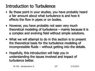
Introduction to Turbulence • By these point in your studies, you have probably heard a fair amount about what turbulence is and how it effects the flow in pipes or on bodies. • However, you have probably not seen very much theoretical modeling of turbulence – mainly because it is a complex and evolving field without simple solutions. • What we will attempt to do in this section is to present the theoretical basis for the turbulence modeling of incompressible fluids – without getting into the details. • Hopefully, this introduction will help you in understanding the issues involved and impact of turbulence better. AE 302 - Aerodynamics II
Introduction to Turbulence [2] • Turbulence is usually characterized by unsteady, chaotic but motion with an underlying well define average. • Thus, the flow variables, and in particular velocity, are functions of time as well as position: • However, because of the existence of an average velocity we can write these velocities as the sum of a steady, time invariant component and a fluctuation one: • Where the average or mean values are defined by the time average: AE 302 - Aerodynamics II
Introduction to Turbulence [3] • Where the length of time used for averaging, T, need only be enough to obtain a good steady mean value. • The fluctuating velocities are then define by the difference: • Note that by definition, the time average of the fluctuating velocities is zero: • Where this idea of splitting the properties into mean and fluctuations is useful is in considering the time averages of our conservation equations. AE 302 - Aerodynamics II
Reynolds Equations • Consider our 2-D, incompressible boundary layer equations that we used for the Blassius solution. • To simplify the following process, let’s rewrite the momentum equation by adding in the continuity equation multiplied by the horizontal velocity, u. • Or, noticing that some of the terms on the left-hand-side can be combined using reverse differentiation by parts… AE 302 - Aerodynamics II
Reynolds Equations [2] • Now, replace the instantaneous velocities with the split sum of mean and fluctuation values: • To give the rather lengthy result: • This hardly seems like an improvement – but now consider time averaging the entire equations. • Any term which involves a product of a fluctuating quantity alone or in product with a mean value vanishes. AE 302 - Aerodynamics II
Reynolds Equations [3] • Only terms with only mean values or products of fluctuating values will remain. • These two new terms can be written in simplified from as: • Thus, the time averaged, or Reynolds averaged momentum equation is: AE 302 - Aerodynamics II
Reynolds Equations [4] • You might wonder why these two new terms do not drop out in the averaging process. • The first term does not average to zero because the product of a fluctuation with itself must be a positive. • Since the integrand can only be positive (or zero), the integration must also yield a positive result. • However, this term, which represents a turbulent axial stress in the flow, is usually quite small and is neglected in normal boundary layer analysis. AE 302 - Aerodynamics II
Reynolds Equations [5] • On the other hand, the term with the product of the x and y velocity fluctuations would have a zero time average if the fluctuations in the two axis were uncorrelated – i.e. they had no relation to each other. • But, in a shear layer, there is a correlation! • A chunk or packet of fluid in one shear layer which has a downward fluctuations, negative v’, arrives at a lower layer with a positive fluctuation, positive u’, relative to the local flow: Initial, t Final, t+dt AE 302 - Aerodynamics II
Reynolds Equations [6] • The reverse occurs for un upward fluctuation, positive v’ but negative u’. • Thus, the integrand will more often be a negative number in a shear layer – and the integration will yield a negative value. • This term is called the turbulent shear stress, or apparent turbulent stress, or simply the Reynolds stress. • This is the additional shear stress we associate with turbulent flow and it can be many orders of magnitude greater than the laminar shear stress. AE 302 - Aerodynamics II
Reynolds Equations [7] • Using the previous discussions then, we arrive at the time averaged conservation equation often called the Reynolds equations: • These equations, or the similar equations in 3-D compressible flow, form the basis of the great majority of turbulent flow analysis with fairly good success. • However, a lot of modern research in turbulence is based upon the modeling the unsteady rather than time-averaged equations. • Apparently, much behavior current models don’t predict well may be due to the very unsteadiness itself. AE 302 - Aerodynamics II
Turbulence Modeling • The impact of turbulence my be thought of as producing an additional, turbulent viscosity similar to its laminar counterpart. I.e.: • This assumption is knows as the Boussinesq analogy. • From the turbulent shear stress equation just derived, it follows that the turbulent stress and viscosity would be: • The field of study called Turbulence Modeling is essentially trying to develop a mathematical model for the above terms that is accurate – and hopefully not to difficult to evaluate. AE 302 - Aerodynamics II
Turbulence Modeling [2] • The difficulty in turbulence modeling is that the turbulent viscosity is a flow property, not a fluid property. • Thus, a good turbulent model would depend upon: • Local flow velocities and velocity gradients. • The history of the flow before the local time and location. • The effects of surface roughness and surface geometry. • Unfortunately, to do all of these, the model will probably not be simply and easy to evaluate. • We will look at two relatively simple models: • Prandlt’s Mixing Length Model • The Baldwin-Lomax Model AE 302 - Aerodynamics II
Prandlt’s Mixing Length Model • Prandlt originally proposed the concept that the velocity perturbations were due to turbulent eddies in the flow. • As a result, the magnitude of the perturbations should depend upon the characteristic size, or length, of the eddies and the gradient in mean velocity. i.e • Thus, the Reynolds stress would be: • Or the turbulent viscosity could be written as: AE 302 - Aerodynamics II
Prandlt’s Mixing Length Model [2] • The absolute value is because the viscosity should always be positive no matter the sign of the gradient. • The task is then to determine reasonable values for the characteristic mixing length, l. • Two important observations help in this regard. • The first is that the mixing length must go to zero at the wall itself since there cannot be flow through the wall. • This leads to the idea of a laminar sub-layer – a region nearest to the wall were there is only laminar stress. • The second observation is that the mixing length in the outer boundary layer approaches a constant value that is some fraction of the boundary layer thickness. AE 302 - Aerodynamics II
Prandlt’s Mixing Length Model [3] • Thus, one mixing length model proposed by van Driest has an inner mixing length given by: • Where and A are two constant which must be specified to correlate with experiment – usually =0.41 and A+=26. • For the outer regions of the boundary layer, the mixing length is assume a constant fraction of the thickness. • Where this new constant is usually taken as: C=0.09. • The model switches from the inner to outer mixing lengths at the height when: AE 302 - Aerodynamics II
Baldwin-Lomax Model • The Prandlt Mixing Length Model with the given values for inner and outer mixing length gives an excellent prediction of the shape of a turbulent velocity profile. • Unfortunately, it doesn’t always give a great correlation to experimental measurements. • A relatively simple and popular modification which improves the correlation is due to Baldwin and Lomax. • They kept the inner mixing length correlation pretty much intact: • With van Driest’s equation for the inner mixing length. AE 302 - Aerodynamics II
Baldwin-Lomax Model [2] • For the outer layer, this model uses a more complex model: • K and Ccp are two constants that will be given shortly. • The function Fwake is selected to find the maximum mixing length that occurs in the BL – its form is: • Where ymax is the height above the wall where Fmax is evaluated – and a new constant Cwk has been introduced. AE 302 - Aerodynamics II
Baldwin-Lomax Model [3] • The other term, known as the Klebanoff intermittency factor accounts for the fact the mixing drops off at the edge of the BL: • As you can see, more complex models attempt to correctly account for more and more of the observed features of turbulent flow. • However, the constants which show up don’t fall out of the sky – they are usually chosen to give the best correlation to experiment. • Common selections for these constants are: AE 302 - Aerodynamics II
Turbulent Conductivity • In addition to the turbulent viscosity, in high speed flows or problems with heat transfer, a turbulent conductivity is needed. • While a separate model could be created for this factor, most researchers take the easy route and relate the viscosity and conductivity through the Prandlt number. • Where experiment has shown that the turbulent Prandlt number is very close to 1.0. AE 302 - Aerodynamics II
Turbulent Flat Plate Flow • Given these turbulence models, I would love to show you some typical solutions. • However, even the simplest solution in turbulent flow – that for a flat plate – is very computationally intensive. • Instead, I will just repeat the time honored flat plate experimental results you have already seen: • Finishing with this result is very appropriate since the whole point of turbulence modeling is to find analytic formulations which will agree with the above. AE 302 - Aerodynamics II