How to solve a large sparse linear system arising in groundwater and CFD problems
160 likes | 332 Vues
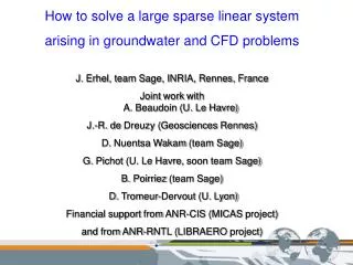
How to solve a large sparse linear system arising in groundwater and CFD problems J. Erhel, team Sage, INRIA, Rennes, France Joint work with A. Beaudoin (U. Le Havre) J.-R. de Dreuzy ( Geosciences Rennes) D. Nuentsa Wakam (team Sage) G. Pichot (U. Le Havre, soon team Sage)

How to solve a large sparse linear system arising in groundwater and CFD problems
E N D
Presentation Transcript
How to solve a large sparse linear system arising in groundwater and CFD problems J. Erhel, team Sage, INRIA, Rennes, France Joint workwithA. Beaudoin (U. Le Havre) J.-R. de Dreuzy (Geosciences Rennes) D. NuentsaWakam (team Sage) G. Pichot (U. Le Havre, soon team Sage) B. Poirriez (team Sage) D. Tromeur-Dervout (U. Lyon) Financial support from ANR-CIS (MICAS project) and from ANR-RNTL (LIBRAERO project)
Ax=b with A non singular and sparse Bad idea: compute A-1then x=A-1 b Good idea: apply a direct or iterativesolver
First case A symmetric positive definite (spd) First example: flow in heterogeneousporous media Second example: flow in 3D discrete fracture networks Second case A non symmetric Example: Navier-Stokes with turbulence
H2OLab software platform Random physical models Fracture Networks MP_FRAC Fractured-Porous Media Porous Media PARADIS Numerical methods GW_NUM Utilitaries GW_UTIL Input / Output Visualization Results structures Parameters structures Parallel and grid tools Geometry Solvers PDE solvers ODE solvers Linear solvers Particle tracker UQ methods Monte-Carlo Open source libraries Boost, FFTW, CGal, Hypre, Sundials, MPI, OpenGL, Xerces-C,…
H2OLab methodology • Optimization and Efficiency • Use of free numerical libraries and own libraries • Test and comparison of numerical methods • Parallel computation (distributed and grid computing) • Genericity and modularity • Object-oriented programming (C++) • Encapsulated objects and interface definitions • Maintenance and use • Intensive testing and collection of benchmark tests • Documentation : user’s guide, developer’s guide • Database of results and web portal • Collaborative development • Advanced Server (Gforge) with control of version (SVN),… • Integrated development environments (Visual, Eclipse) • Cross-platform software (Cmake, Ctest) • Software registration and future free distribution
First case A symmetric positive definite (spd) arising from an elliptic or parabolic problem Flow equations of a groundwater model Q = - K*grad (h) in Ω div (Q) = 0 in Ω Boundary conditions on ∂Ω Spatial discretization scheme Finite element method or finite volume method … Ax=b, with A spd and sparse
Nul flux Fixed head Fixed head Nul flux An example of domain and data Heterogeneous porous media 2D Heterogeneous permeability field Stochastic model Y = ln(K) with correlation function
Numerical method for 2D heterogeneous porous medium Finite Volume Method with a regular mesh Large sparse structured matrix of order N with 5 entries per row
First solver for A spd and elliptic Direct method based on Cholesy factorization Cholesky factorization A=LDLT with L lower triangular and D diagonal Based on elimination process Fill-in in L L sparse but not as much as A More memory and time Due to fill-in
Fill-in in Cholesy factorization depends on renumbering Symmetric renumbering PT A P = LDLT with P permutation matrix L full matrix L as sparse as A: no fill-in
Analysis of fill-in with elimination tree Matrix graph and interpretation of elimination j connected to i1,i2 and i3 in the graph Elimination tree All steps of elimination in Cholesky algorithm
Sparse Cholesky factorization Symbolic factorization Build the elimination tree Reduction of fill-in Renumber the unknowns with matrix P minimum degree algorithm Nested dissection algorithm Numerical factorization Build the matrices L and D Six variants of the nested three loops Two column-oriented variants: left-looking and right-looking Use of BLAS3 thanks to a multifrontal or supernodal technique
Sparse direct solver (here PSPASES) applied to heterogeneous porous media Fill-in CPU time Theory : NZ(L) = O(N logN) Theory : Time = O(N1.5)
Parallel Monte-Carlo results • Cluster of nodes with a Myrinet network • Each node is one-core bi-processor, with 2Go memory • Monte-Carlo run of flow and transport simulations • Computational domain of size 1024x1024