Download
1 / 27
290 likes | 890 Vues
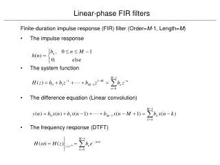
Linear-phase FIR filters. Finite-duration impulse response (FIR) filter (Order= M -1, Length= M ) The impulse response The system function The difference equation (Linear convolution) The frequency response (DTFT). Linear-phase FIR filters.

E N D
Linear-phase FIR filters • Finite-duration impulse response (FIR) filter (Order=M-1, Length=M) • The impulse response • The system function • The difference equation (Linear convolution) • The frequency response (DTFT)
Linear-phase FIR filters • Linear-phase FIR filter (Order=M-1, Length=M) • = 0, /2. is a constant • Four types
Linear-phase FIR filters • Type-1 linear-phase FIR filter (Symmetrical, M odd) • = 0. = (M-1)/2 (integer) • Symmetric about (the index of symmetry)
Linear-phase FIR filters • Type-2 linear-phase FIR filter (Symmetrical, M even) • = 0. = (M-1)/2 (non-integer)
Linear-phase FIR filters • Type-3 linear-phase FIR filter (Antisymmetrical, M odd) • = /2. = (M-1)/2 (integer)
Linear-phase FIR filters • Type-4 linear-phase FIR filter (Antisymmetrical, M even) • = /2. = (M-1)/2 (non-integer)
Design Specs (LPF) • Band [0,p]: pass band • Band [s, ]: stop band • Band [p, s]: transition band • 1: Absolute ripple in pass band • 2: Absolute ripple in stop band • Rp: Relative ripple in pass band (in dB) • As: Relative ripple in stop band (in dB) FIR LPF filter specifications: (a) Absolute (b) Relative
w p Ideal LPF c= /4-shifted w p Ideal LPF c= /4 0.25 0.25 0.2 0.2 0.15 0.15 0.1 0.1 0.05 0.05 0 0 -0.05 -0.05 -0.1 -0.1 -30 -20 -10 0 10 20 30 -30 -20 -10 0 10 20 30 Window Design Techniques Shifting
Window Design Techniques • General Design Procedures: • : Ideal frequency response (given) • Step 1 • Step 2 • Step 3 • Window function • symmetric about over • 0 otherwise
Window Design Techniques Rectangular Window • Exact transition width = s - p = 1.8/M • Min. stopband attenuation = 21dB • MATLAB function: w=boxcar (M)
Window Design Techniques Bartlett Window • Exact transition width = s - p = 6.1/M • Min. stopband attenuation = 25dB • MATLAB function: w=bartlett (M)
Window Design Techniques Hann Window • Exact transition width = s - p = 6.2/M • Min. stopband attenuation = 44dB • MATLAB function: w=hann (M)
Window Design Techniques Hamming Window • Exact transition width = s - p = 6.6/M • Min. stopband attenuation = 53dB • MATLAB function: w=hamming (M)
Window Design Techniques Blackman Window • Exact transition width = s - p = 11/M • Min. stopband attenuation = 74dB • MATLAB function: w=blackman (M)
Window Design Techniques LPF Design function hd=ideal_lp(wc,M) %hd: ideal LPF impulse response between 0 and M-1 %wc: cut-off frequencies in radians %M: length of the filter alpha=(M-1)/2; n=[0:M-1]; m=n-alpha; fc=wc/pi; hd=fc*sinc(fc*m);
Window Design Techniques LPF Design Example: p=0.2 s=0.3 As=50 dB %Example 1 in FIR filter design wp=0.2*pi; ws=0.3*pi; tr_width=ws-wp; M=ceil(6.6*pi/tr_width)+1; n=[0:M-1]; wc=(ws+wp)/2; %ideal cutoff frequency hd=ideal_lp(wc,M); w_hamming=(hamming(M))'; h=hd.*w_hamming; figure(1);stem(n,h); title('h(n)') figure(2);freqz(h,[1])
Window Design Techniques BPS example: 1s=0.2, 1p=0.35, 2p=0.65, 2s=0.8 As=60 dB Two transition band widths must be the same!
Window Design Techniques %Example 2 in FIR filter design % BPS design wp1=0.35*pi; ws1=0.2*pi; wp2=0.65*pi; ws2=0.8*pi; %only one transition bandwidth allowed in window design tr_width=min(wp1-ws1,ws2-wp2); M=ceil(11*pi/tr_width)+1; n=[0:M-1]; wc1=(ws1+wp1)/2; %ideal cutoff frequency 1 wc2=(ws2+wp2)/2; %ideal cutoff frequency 2 hd=ideal_lp(wc2,M)-ideal_lp(wc1,M); w_blackman=(blackman(M))'; h=hd.*w_blackman; figure(1);stem(n,h); title('h(n)') figure(2);freqz(h,[1])
Window Design Techniques Example: Digital differentiator %Example 2 in FIR filter design % Digital differentiator design M=21;alpha=(M-1)/2;n=0:M-1; hd=(cos(pi*(n-alpha)))./(n-alpha);hd(alpha+1)=0; w_ham=(hamming(M))'; h=hd.*w_ham; [H,W]=freqz(h,[1]); plot(W/pi,abs(H)); title('Digital differentiator: |H(\omega)|')
Window Design Techniques >> t=linspace(-2,2,1000); >> xt=sin(2*pi*t);yt=conv(xt,h); >> subplot(2,1,1);plot(xt);title('x(t)=sin(2\pit)') >> subplot(2,1,2);plot(yt(22:end));title('y(t)=Dx(t)')