Download
1 / 26
270 likes | 504 Vues
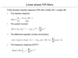
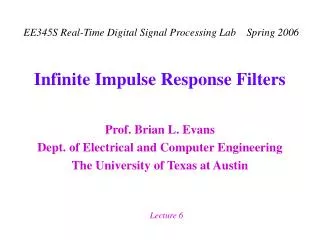
Infinite Impulse Response Filters. Digital IIR Filters. Infinite Impulse Response (IIR) filter has impulse response of infinite duration, e.g. How to implement the IIR filter by computer? Let x [ k ] be the input signal and y [ k ] the output signal,. Z.

E N D
Digital IIR Filters • Infinite Impulse Response (IIR) filter has impulse response of infinite duration, e.g. • How to implement the IIR filter by computer? Let x[k] be the input signal and y[k] the output signal, Z Recursively compute output, given y[-1] and x[k]
Difference equation Recursive computation needs y[-1] and y[-2] For the filter to be LTI,y[-1] = 0 and y[-2] = 0 Transfer function Assumes LTI system Block diagram representation Second-order filter section (a.k.a. biquad) with 2 poles and 0 zeros x[k] y[k] UnitDelay 1/2 y[k-1] UnitDelay 1/8 y[k-2] Different Filter Representations Poles at –0.183 and +0.683
v[k] x[k] b0 y[k] UnitDelay a1 b1 v[k-1] UnitDelay v[k-2] a2 b2 Digital IIR Biquad • Two poles and zero, one, or two zeros • Take z-transform of biquad structure • Real coefficients a1, a2, b0, b1, and b2 means poles and zeros in conjugate symmetric pairs a± j b
Digital IIR Filter Design • Poles near unit circle indicate filter’s passband(s) • Zeros on/near unit circle indicate stopband(s) • Biquad with zeros z0 and z1, and poles p0 and p1 Transfer function Magnitude response |a – b| is distance between complex numbers a and b Distance from point on unit circle ej and pole location p0
Im(z) Im(z) Im(z) O O X X X O Re(z) Re(z) Re(z) O X X X O O Digital IIR Biquad Design Examples • Transfer function • Poles (X) & zeros (O) in conjugate symmetric pairs • For coefficients in unfactored transfer function to be real • Filters below have what magnitude responses? lowpasshighpass bandpass bandstop allpass notch?
A Direct Form IIR Realization • IIR filters having rational transfer functions • Direct form realization • Dot product of vector of N +1coefficients and vector of currentinput and previous N inputs (FIR section) • Dot product of vector of M coefficients and vector of previous M outputs (FIR filtering of previous output values) • Computation: M + N + 1 MACs • Memory: M + N words for previous inputs/outputs andM + N + 1 words for coefficients
x[k] y[k] b0 UnitDelay UnitDelay a1 b1 x[k-1] y[k-1] UnitDelay UnitDelay aM a2 bN b2 x[k-2] y[k-2] Feed-forward Feedback UnitDelay UnitDelay x[k-N] y[k-M] Filter Structure As a Block Diagram Note that M and N may be different
Another Direct Form IIR Realization • When N = M, • Here, Wm(z) = bmX(z) + am Y(z) • In time domain, • Implementation complexity • Computation: M + N + 1 MACs • Memory: M + N words for previous inputs/outputs andM + N + 1 words for coefficients • More regular layout for hardware design
b0 a1 b1 aM a2 bN b2 Filter Structure As a Block Diagram x[k] y[k] UnitDelay UnitDelay x[k-1] y[k-1] UnitDelay UnitDelay x[k-2] y[k-2] Feed-forward Note that M = N impliedbut can be different Feedback UnitDelay UnitDelay x[k-N] y[k-M]
Yet Another Direct Form IIR • Rearrange transfer function to be cascade of an an all-pole IIR filter followed by an FIR filter • Here, v[k] is the output of an all-pole filter applied to x[k]: • Implementation complexity (assuming MN) • Computation: M + N + 1 = 2 N + 1 MACs • Memory: M + 1 words for current/past values of v[k] andM + N + 1 = 2 N + 1 words for coefficients
v[k] x[k] b0 y[k] UnitDelay a1 b1 v[k-1] UnitDelay v[k-2] a2 b2 Feed-forward Feedback UnitDelay v[k-M] aM bN Filter Structure As Block Diagram Note that M = N impliedbut they can be different M=2 yields a biquad
Demonstrations (DSP First) • Web site: http://users.ece.gatech.edu/~dspfirst • Chapter 8: IIR Filtering Tutorial (Link) • Chapter 8: Connection Betweeen the Z and Frequency Domains (Link) • Chapter 8: Time/Frequency/Z Domain Moves for IIR Filters (Link)
Review Stability • A digital filter is bounded-input bounded-output (BIBO) stable if for any bounded input x[k] such that | x[k] | B < , then the filter response y[k] is also bounded | y[k] | B < • Proposition: A digital filter with an impulse response of h[k] is BIBO stable if and only if • Any FIR filter is stable • A rational causal IIR filter is stable if and only if its poles lie inside the unit circle
Review Stability • Rule #1: For a causal sequence, poles are inside the unit circle (applies to z-transform functions that are ratios of two polynomials) OR • Rule #2: Unit circle is in the region of convergence. (In continuous-time, imaginary axis would be in region of convergence of Laplace transform.) • Example: Stable if |a| < 1 by rule #1 or equivalently Stable if |a| < 1 by rule #2 because |z|>|a| and |a|<1 pole at z=a
Z and Laplace Transforms • Transform difference/differential equations into algebraic equations that are easier to solve • Are complex-valued functions of a complex frequency variable Laplace: s = + j 2 f Z: z = rej • Transform kernels are complex exponentials: eigenfunctions of linear time-invariant systems Laplace: e– s t = e– t –j 2 f t = e– t e – j 2 f t Z: z–k = (rej)–k= r–ke– jk dampening factor oscillation term
f[k] H(z) y[k] Z Laplace H(s) Z and Laplace Transforms • No unique mapping from Z to Laplace domain or from Laplace to Z domain • Mapping one complex domain to another is not unique • One possible mapping is impulse invariance • Make impulse response of a discrete-time linear time-invariant (LTI) system be a sampled version of the continuous-time LTI system.
Im{z} 1 Re{z} Impulse Invariance Mapping • Impulse invariance mapping is z = e s T Im{s} 1 Re{s} -1 1 -1 s = -1 j z = 0.198 j 0.31 (T = 1 s) s = 1 j z = 1.469 j 2.287 (T = 1 s)
f[k] H(z) y[k] Z Laplace H(esT) Optional Impulse Invariance Derivation
Analog IIR Biquad • Second-order filter section with 2 poles and 2 zeros • Transfer function is a ratio of two real-valued polynomials • Poles and zeros occur in conjugate symmetric pairs • Quality factor: technology independent measure of sensitivity of pole locations to perturbations • For an analog biquad with poles at a ±jb, where a < 0, • Real poles: b = 0 so Q = ½ (exponential decay response) • Imaginary poles: a = 0 so Q = (oscillatory response)
Analog IIR Biquad • Impulse response with biquad with poles a ±jb with a < 0 but no zeroes: • Pure sinusoid when a = 0 and pure decay when b = 0 • Breadboard implementation • Consider a single pole at –1/(R C). With 1% tolerance on breadboard R and C values, tolerance of pole location is 2% • How many decimal digits correspond to 2% tolerance? • How many bits correspond to 2% tolerance? • Maximum quality factor is about 25 for implementation of analog filters using breadboard resistors and capacitors. • Switched capacitor filters: Qmax 40 (tolerance 0.2%) • Integrated circuit implementations can achieve Qmax 80
Digital IIR Biquad • For poles at a ±jb = r e ± j , where is the pole radius (r < 1 for stability), with y = –2 a: • Real poles: b = 0 so r = | a | and y = ±2 r which yields Q = ½ (exponential decay response C0an u[n] + C1n an u[n]) • Poles on unit circle: r = 1 so Q = (oscillatory response) • Imaginary poles:a = 0 so y = 0 so • 16-bit fixed-point DSPs: Qmax 40 (extended precision accumulators)
Analog/Digital IIR Implementation • Classical IIR filter designs Filter of order n will have n/2 conjugate roots if n is even or one real root and (n-1)/2 conjugate roots if n is odd Response is very sensitive to perturbations in pole locations • Robust way to implement an IIR filter Decompose IIR filter into second-order sections (biquads) Cascade biquads in order of ascending quality factors For each pair of conjugate symmetric poles in a biquad, conjugate zeroes should be chosen as those closest in Euclidean distance to the conjugate poles
Classical IIR Filter Design • Classical IIR filter designs differ in the shape of their magnitude responses Butterworth: monotonically decreases in passband and stopband (no ripple) Chebyshev type I: monotonically decreases in passband but has ripples in the stopband Chebyshev type II: has ripples in passband but monotonically decreases in the stopband Elliptic: has ripples in passband and stopband • Classical IIR filters have poles and zeros, except that analog lowpass Butterworth filters are all-pole • Classical filters have biquads with high Q factors
Analog IIR Filter Optimization • Start with an existing (e.g. classical) filter design • IIR filter optimization packages from UT Austin (in Matlab) simultaneously optimize Magnitude response Linear phase in the passband Peak overshoot in the step response Quality factors • Web-based graphical user interface (developed as a senior design project) available at http://signal.ece.utexas.edu/~bernitz
Original Optimized Analog IIR Filter Optimization • Design an analog lowpass IIR filter with dp = 0.21 at wp = 20 rad/s and ds = 0.31 at ws = 30 rad/s with Minimized deviation from linear phase in passband Minimized peak overshoot in step response Maximum quality factor of second-order sections is 10 Linearized phase in passband Minimized peak overshoot initial optimized