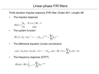
Impulse Response Measurement and Equalization
Impulse Response Measurement and Equalization. Digital Signal Processing LPP Erasmus Program Aveiro 2012. Impulse response measurement. Measurement of impulse responses is a common task in different areas (specially important in audio processing).

Impulse Response Measurement and Equalization
E N D
Presentation Transcript
Impulse Response Measurement and Equalization Digital SignalProcessing LPP Erasmus Program Aveiro 2012
Impulse response measurement Measurement of impulse responses is a common task in different areas (specially important in audio processing) Typically, PC hardware is used to perform this task using the following setup: x(t) x[n] DAC h(t) y[n] ADC PC y(t) The following assumptions are made: The whole system between x[n] and y[n] shows time-invariant behaviour. All involved components are sufficiently linear The impulse response can be considered finite (h[n]≈0 for n > M)
Impulse response measurement In theory, any input signal can be used to measure the impulse response of a linear system. The output signal can be expressed in terms of this impulse response by: Assuming that the impulse response only has N significant samples, the former equation can be rewritten in matrix form as: where L is the length of the input signal
Impulse response measurement Then, the impulse response can be theoretically obtained as: where X-1* represents the pseudo-inverse of matrix X: (XT·X)-1·XTor XT·(X·XT)-1 However, in practice, very long input signals would be needed to attain high suppression of measurement noise, resulting in extremely large problems which may turn out to become computationally intractable.
Impulse response measurement An atractive approach consist in using as input signal one whose auto-correlation function is similar to a delta sequence: In this case, the impulse response of the system can be obtained by cross-correlating the output and the input signals:
Impulse response measurement Assuming that the length of the input signal is K and that the impulse response has only N significant samples, we have:
Impulse response measurement Using this indirect approach, a great inmunity against noise is achieved: • The energy of the input signal can be as large as desired, since we have just to extend its duration. • As noise corrupting the output signal is uncorrelated with the input signal x, its contribution in the measurement of the impulse response is very small:
Impulse response measurement Typical test signals: x(t) Rxx(t) Chirp (Continuous-time frequency varying sinusoid) PR sequence (13-bit Barker Code) White Gaussian Noise
Impulse response equalization An Equalizer is a system whose main objective is to undo the effect of a previous stage, typically a transmission channel: Channel c[n] Equalizer g[n] + Ideally, the composite impulse response of the channel and the equalizer is a delta (flat frequency response), so that the output of the equalizer is a delayed version of the input signal. We can distinguish between two types of equalizers: Fixed equalizers (its coefficients do not change with time) Adaptive equalizers (its coefficients are updated periodically based on the current channel characteristics)
Impulse response equalization Fixed Equalizer (Zero-Forcing) In zero-forcing equalization, the equalizer response g[n] attempts to completely inverse the channel by forcing : Or using matrix representation:
Impulse response equalization Adaptive Equalizer When the channel is time-varying (LTV), it is necessary to update the equalizer coefficients in order to track the channel changes. Define the input signal to the equalizer as a vector ck where: and an equalizer weight vector gk, where Then, the output signal is given by: And the error signal ek is given by:
Impulse response equalization Adaptive Equalizer An adaptive channel equalizer has the following structure.
Impulse response equalization Adaptive Equalizer The least mean-square (LMS) algorithm carries out the mean squared error by recursively updating the coefficients using the following rules: The step parameter a, controls the adaptation rate and must be chosen carefully to guarantee convergence. The equalizer is converged if the error ek becomes steady.