STAT131 Week7 L1a Exponential Distribution
STAT131 Week7 L1a Exponential Distribution. Anne Porter alp@uow.edu.au. Lecture Outline. Review Poisson Introduction to the Exponential Context/assumptions Probability Centre Spread Calibration of the model Goodness of fit. Poisson. Video Clip : Blowhole.


STAT131 Week7 L1a Exponential Distribution
E N D
Presentation Transcript
STAT131Week7 L1aExponential Distribution Anne Porter alp@uow.edu.au
Lecture Outline • Review Poisson • Introduction to the Exponential • Context/assumptions • Probability • Centre • Spread • Calibration of the model • Goodness of fit
Poisson • Video Clip : Blowhole
Poisson: The random variable of interest , X, is the number of events occurring in a fixed dimension of length t. • The events occur in time or along any other dimensional continuum. • In each infinitesimally small period of length the probability of an event is P(event)= for some value . • In any infinitesimally small period of length, , the probability of two or more events is zero ie two events do not occur simultaneously. • The co-occurrence of events in any two non-overlapping periods is independent. • (Griffiths et al, 1998)
Exponential distribution • How else can we think about the count data we examined as exemplifying the Poisson distribution? • The time until the first event occurs and because • the exponential process has no memory of the previous event • The time until the next event or • The time between events.
Context or Problem - Exponential • Given a Poisson process observed from time t=0 with a rate of events . Let Y be the time when the first event occurs. Then Y has an exponential distribution with parameter . Any two successive events also has an exponential distribution with parameter .
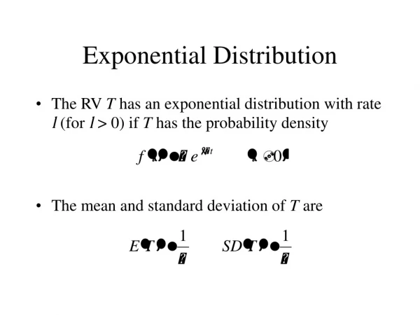
Probability:Exponential The probability that the random event Y takes on a value between time1 and time 2 is given by =
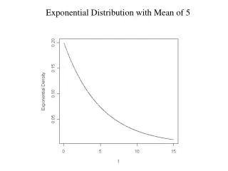
Centre:Exponential • The mean of the Exponential() Random Variable Y is given as
Spread: Variance Spread: Variance
Calibration of the Exponential Model • To estimate based on a sample we set the mean of the distribution equal to the sample mean that is so
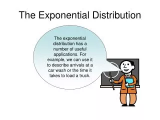
Problem • The random variable of interest is time to a the next car passing.The count of cars per 30 second interval is an homogenous Poisson (). • The data consist of a list of inter-car arrival times in seconds. • Develop a model to describe the data
Suggesting a model • Context and assumptions • Exploratory data analysis to reveal If we have a homogeneous Poisson process with a rate of events per unit of time then the time from t=0 to the first event is a random variable with an exponential distribution. Centre, shape, spread, outliers, allow examination of theoretical assumptions What plot might be useful?
Stem- and leaf plot reveals an exponential distribution(12 bins) • Frequency Stem & Leaf • 7.00 0 * 2223333 • 34.00 0 . 5555556666666777778888899999999999 • 18.00 1 * 000111122223333444 • 9.00 1 . 555567889 • 12.00 2 * 001222223344 • 4.00 2 . 5678 • 6.00 3 * 011123 • 7.00 3 . 6777899 • 3.00 4 * 133 • 2.00 4 . 59 • 2.00 5 * 22 • 1.00 5 . 9 • 7.00 Extremes (64), (68), (72), (74), (86), (93) • Stem width: 10 • Each leaf: 1 case(s) Exponential shape Centre Spread Outliers
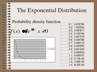
Histogram suggests and exponential shaped distribution (20 class intervals or bins) Little jagged rather than smooth so try fewer bins
Exponential shape Histogramsuggests and exponential shaped distribution (10 class intervals or bins)
How many bins should we use? • let the data speak for themselves experiment • balance between too smooth and too jagged to reveal shape
Exploratory statistics TIME inter-arrival time (secs) Valid cases: 112.0 Missing cases: .0 Percent missing: .0 Mean 21.0982 Std Err 1.8138 Min 2.0000 Skewness 1.6881 Median 13.5000 Variance 368.4858 Max 93.0000 S E Skew .2284 5% Trim 18.9623 Std Dev 19.1960 Range 91.0000 Kurtosis 2.6822 IQR 21.5000 S E Kurt .4531
Exploratory statistics: Compare Mean and Standard deviation Theoretically and That is In our sample the mean =21.0982 and the standard deviation=19.1960 These are close about 9% difference as a percentage of the mean
Exploratory statistics: Calibration What should we do to calibrate the model? This gives Estimate ?
Probabilities • To find the probability of the time to be within a certain time interval we use • where • P(0<Y<20) = • P(20<Y<40) = • P(40<Y<60) = • P(60<Y<80) = • P(Y>80) =
Probabilities • To find the probability of the time to be within a certain time interval we use • where • P(0<Y<20) = e -0.047x0-e -0.047x20 = e0-e-0.94 = 1-0.3906 =0.6094
Probabilities • P(0<Y<20) = 1- 0.3906 = 0.6094 • P(20<Y<40) = = e -0.047x20 -e-0.047x40 = 0.3906-0.1526 =0.2380
Probabilities • P(0<Y<20) = 1- 0.3906 = 0.6094 • P(20<Y<40) = 0.3906 - 0.1526 = 0.2380 • P(40<Y<60) = 0.1526 - 0.0596 = 0.0930 • P(60<Y<80) = 0.0595 - 0.0233 = 0.0362 • P(Y>80) =1-(0.6094+0.2380+0.0930+0.0362) =0.0234
Expected counts • To find the frequencies of inter-arrival times expected in each class interval Multiply the probability of falling in an interval by the total number of inter-arrival times • freq expected (0<Y<20) = 0.6094 x 112= 68.25
Finding expected counts for cells • freq expected (0<Y<20) = 0.6094 x 112= 68.25 • freq expected (20<Y<40) = 0.2380 x112 = 26.66 • freq expected (40<Y<60) = 0.0930 x 112 = 10.42 • freq expected (60<Y<80) = 0.0362 x 112 = 4.05 • freq expected (Y>80) = 112-(68.25+26.66+10.42+4.05)=2.62 As the expected number in the last two intervals amount to less than 5 amalgamate these cells to have freq expected >60 =6.67
Finding expected counts for cells • freq expected (0<Y<20) = 0.6094 x 112= 68.25 • freq expected (20<Y<40) = 0.2380 x112 = 26.66 • freq expected (40<Y<60) = 0.0930 x 112 = 10.42 • freq expected (Y>60) = 6.67 112.00 • As the expected number in the last two intervals amount to less than 5 we will amalgamate these cells to have freq expected >60 = 112- (68.25+26.66+10.42) =6.67
(0-E)2 E • class interval freq freq Observed Expected • (0<Y<20) 68 68.25 • (20<Y<40) 29 26.66 • (40<Y<60) 8 10.42 • Y>60 76.67 • total 0.0009 0.2054 0.5620 0.016 0.7846 112 112
Decision • 0.7486 <g-p-1 ie < 4-1-1 so the data can be considered to fit the model • Informal: Where we have one parameter l and g= 4 cells and d=g-p-1=2. If > there is evidence of lack of fit BUT 0.7486< 2+4 so there is little evidence that the data do not fit the model
Decision • Formal > tabulated value (5.991)with a=0.05 and df=g-p-1 then there is evidence the data do not fit the model • As 0.7486<5.991 there is little evidence of lack of fit between the exponential (.047) model and the data
Assess Fit:Observed compared to Expected (Need to calculate probabilities and expected counts first and this has been done with 5 not 4 bins as most appropriate Given in the last cell the expected count is too small) Good fit likely
Simulation • Simulate many samples of the same size (n=112) • Simulate them so as to have the same parameter(s) • In this case =0.047 • See if the data set is similar to those samples simulated and known to come from an exponential model (0.047) • Same bins is sensible • If the data set is typical of those simulated it is likely that the data follow the exponential (0.047) model
Simulate Exponential (0.047) (n=112 as per original data set)Simulated samples can be generated in SPSS
Simulate Exponential (0.047) (n=112 as per original data set)
Simulate Exponential (0.047) (n=112 as per original data set)
Simulate Exponential (0.047) (n=112 as per original data set)
Simulate Exponential (0.047) (n=112 as per original data set)
Simulate Exponential (0.047) (n=112 as per original data set)
Simulate Exponential (0.047) (n=112 as per original data set)
Simulation • If the data set is similar to those samples simulated and known to come from an exponential model () then it is likely that the data set also comes from that same population
Quantile Plots When the points fall on the straight line y(i) =qi where the qi are the quantiles expected with the exponential ().
Quantile - quantile plots • Sort (&enter) the data in ascending order • Determine q1, q2,..qn such that the data are divided into n+1 areas • F(q1)=1/(n+1) = 1/113 • F(q2)=2/(n+1) = 2/113 etc • Find P(0<Y<qi) • Solve for qi • F(q1)= 1/113 = • F(qi)= i/113 = etc • Find P(0<Y<qi) and solve for qi (See lecture notes)
What do we do if the data does not fit the model? • If the model does not fit, ask 'why not?' Could it be that one or more assumptions do not hold. • Look at changes over time, constant rate or lack of independence in time periods • Examine which cells have the largest lack of fit • Look at theoretical relationships eg mean=variance or mean=standard deviation where they exist
Poisson link to the ExponentialNext lecture No events between time zero and time t Is the same as The time of the first event is greater than t