Download

1 / 23
230 likes | 497 Vues
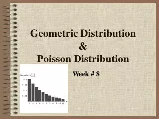
STAT131 Week 5 Lecture 2 Poisson distribution. Anne Porter alp@uow.edu.au. How might the eruptions of the blowhole be measured?. How might the eruptions of the blowhole be measured?. Number of eruptions per minute or per 15 seconds Time between eruptions Time to the next eruption.

E N D
STAT131Week 5 Lecture 2 Poisson distribution Anne Porter alp@uow.edu.au
How might the eruptions of the blowhole be measured? • Number of eruptions per minute or per 15 seconds • Time between eruptions • Time to the next eruption
Poisson distribution: assumptions • When the random variable X of interests is say the number of occurrences of a certain phenomenon (eg eruptions of the blowhole) for a length of time , t then the variable is Poisson distributed if: • in a sufficiently short length of time (say), only 0 or 1 eruptions can happen(>2 is impossible). • the probability that exactly one occurrence happens is proportional to the length of the interval • the numbers of occurrences in non overlapping time intervals are independent
Similarity to Binomial • It is a counting distribution • It is used as a probability model for random experiments which satisfy a different set of assumptions • The Poisson distribution is appropriate when the random variable of interest is the count of the number of times some phenomenon occurs in a fixed period of time, provided the phenomenon occurs ‘at random’ over the time period (Griffiths, 1999)
What questions will we ask about the Random variable? • Probability of some event P(X=x) • Centre of Distribution E(X) • Variance (X) ie 2 • Standard deviation (X) If we have data • How can we calibrate the model • Do the data fit the model
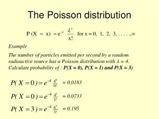
e is the function e on your calculator Probability: P(X=x) • The variable X is distributed according to the function for x= 0, 1,2,…. Where is the rate of occurrence of the phenomenon per unit time
Function e on calculator . =multiply by Example: P(X=x) • If the rate of eruptions is 2 per 15 seconds then 1) what is P(X=0) per unit of time? What is the unit of time? t=1 ie 1 lot of 15 seconds If the question was find P(X=0) in a 1 minute period what would t be? t=4
. =multiply by Example: P(X=x) • If the rate of eruptions is 2 per 15 seconds then 1) what is P(X=1) per unit of time?
Example: P(X=x) If the rate of eruptions is 2 per 15 seconds then 1) what is P(X>1) per unit of time? P(X>1)=1-(P(X=0)+P(X=1)) =1-(0.135+0.271) =0.594 per 15 second interval
Defining the Discrete Random Variable • What do we need to define the discrete random variable x, the number of eruptions in a 15 second interval? Values x and the associated probabilities What must the probabilities sum to? 1
P(X=x) 0 1 2 3 4 5 6 7 8+ X Note the last cell is the rest of the probabilities Define the DRV: Poisson(2) x P(X=x) 0 0.1353 1 0.2707 2 0.2707 3 0.1804 4 0.0902 5 0.0361 6 0.0120 7 0.0034 8+ 0.0012
Per 1 unit of time which is 15 seconds Mean E(X) x P(X=x) x.P(X=x) 0 0.1353 0.0000 1 0.2707 0.2707 2 0.2707 0.5414 3 0.1804 0.5412 4 0.0902 0.3608 5 0.0361 0.1805 6 0.0120 0.0720 7 0.0034 0.0238 8+ 0.00120.0088 • Or E(X) for Poisson=t = 2x1= 2 Sum should equal 2 Rounding 8+ category
e is the function e on your calculator Probability: P(X=x) • Using E(X)==t we can use the modified version of the formulae to find P(X=x) for x= 0, 1,2,…. Where is the rate of occurrence of the phenomenon per unit time
Var(X)=s2 • Var(X)= E[X2]-(E(X))2 • OR • Var(X)=t =2x1 Note theoretically we expect the E[X] to equal the Variance In practice we expect them to be similar and we can compare The mean and variance in samples to see if they are similar When we assess whether the data are likely to fit a Poisson model
Standard deviation X= • ie =1.414 eruptions per 15 seconds
Example: P(X=x) If the rate of eruptions is 2 per 15 minutes then 1) what is P(X=0) per minute? Do you think it would be larger or smaller than P(X=0) per ¼ minute? =.00033546 Note the calculator may have used scientific notation ie 3.3546-04 which is an abbreviation for 3.3546x10 -04
If we were given a data set what other questions would we ask? • Can we calibrate the model to get an estimate for ? • Does the data we have appear to fit the Model • as specified or • as we have calibrated it to be?
Calibrate the model • Choose to make equal to t • If the data are used to estimate the value of • Then when calculating df =g-p-1 for • p is 1 when the estimated from the data
Model fit • Use a Bar chart to compare observed and expected frequencies • Compare observed and expected frequencies • Calculate and use • Informally • Formally • And see if this is too big for the data to fit the model
Another example • What do we have in this clip of cars?
Another example Cars going in two directions • What do we have in this clip of cars? Potentially two Poisson processes And if we measure by the time to the next car or time between cars? Potentially Two exponential processes
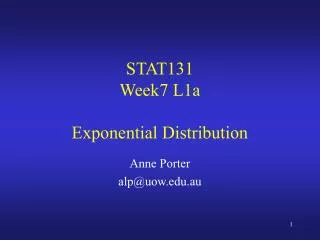
Exponential Distribution • When we have a homogeneous Poisson process with the rate of events per unit time. If the Poisson process is observed from t=0, and Y is the time until the first event occurs then Y has an exponential distribution. We will continue in later lectures examining the exponential distribution