
Uploaded by
asabi
0 SLIDES
364 VUES
10LIKES
Cache
DESCRIPTION
Cache. 2010. 09. 14. Agenda. Cache (9/14) Basic functions Single core cache performance optimization Cache coherency for multi-core Virtual Memory (9/27) Practice (9/27) Running a cycle-accurate simulation model Performance analysis Parameters (cache sizes)
Download

1 / 0
Télécharger la présentation 
Cache
An Image/Link below is provided (as is) to download presentation
Download Policy: Content on the Website is provided to you AS IS for your information and personal use and may not be sold / licensed / shared on other websites without getting consent from its author.
Content is provided to you AS IS for your information and personal use only.
Download presentation by click this link.
While downloading, if for some reason you are not able to download a presentation, the publisher may have deleted the file from their server.
During download, if you can't get a presentation, the file might be deleted by the publisher.
E N D
Presentation Transcript
-
Cache
2010. 09. 14 - Agenda Cache (9/14) Basic functions Single core cache performance optimization Cache coherency for multi-core Virtual Memory (9/27) Practice (9/27) Running a cycle-accurate simulation model Performance analysis Parameters (cache sizes) Prefetch methods (strided, delta correlations)
- [Source: K. Asanovic, 2008] Processor-DRAM Gap (latency) µProc 60%/year 1000 CPU “Moore’s Law” Processor-Memory Performance Gap:(grows 50% / year) 100 Performance 10 DRAM 7%/year DRAM 1 1988 1986 1987 1989 1990 1991 1992 1993 1994 1995 1996 1980 1981 1982 1983 1984 1985 1997 1998 1999 2000 Time Four-issue 2GHz superscalar accessing 100ns DRAM could execute 800 instructions during time for one memory access!
- [Source: J. Kubiatowicz, 2000] What is a cache? Small, fast storage used to improve average access time to slow memory. Exploits spatial and temporal locality In computer architecture, almost everything is a cache! Registers a cache on variables First-level cache a cache on second-level cache Second-level cache a cache on memory Memory a cache on disk (virtual memory) TLB a cache on page table Branch-prediction a cache on prediction information? Proc/Regs L1-Cache Bigger Faster L2-Cache Memory Disk, Tape, etc.
- [Source: K. Asanovic, 2008] n loop iterations subroutine call subroutine return argument access vector access scalar accesses Typical Memory Reference Patterns Address Instruction fetches Spatial locality Temporal & Spatial locality Stack accesses Temporal locality Spatial locality Data accesses Time Temporal locality
- [Source: K. Asanovic, 2008] Temporal Locality Spatial Locality Memory Reference Patterns Memory Address (one dot per access) Time Donald J. Hatfield, Jeanette Gerald: Program Restructuring for Virtual Memory. IBM Systems Journal 10(3): 168-192 (1971)
- [Source: K. Asanovic, 2008] A Typical Memory Hierarchy c.2008 Split instruction & data primary caches (on-chip SRAM) Multiple interleaved memory banks (off-chip DRAM) L1 Instruction Cache Unified L2 Cache Memory CPU Memory Memory L1 Data Cache RF Memory Multiported register file (part of CPU) Large unified secondary cache (on-chip SRAM)
- [Source: K. Asanovic, 2008] Itanium-2 On-Chip Caches(Intel/HP, 2002) Level 1, 16KB, 4-way s.a., 64B line, quad-port (2 load+2 store), single cycle latency Level 2, 256KB, 4-way s.a, 128B line, quad-port (4 load or 4 store), five cycle latency Level 3, 3MB, 12-way s.a., 128B line, single 32B port, twelve cycle latency L3 and L2 caches occupy more than 2/3 of total area!
- [Source: K. Asanovic, 2008] Workstation Memory System(Apple PowerMac G5, 2003) Dual 2GHz processors, each has: 64KB I-cache, direct mapped 32KB D-cache, 2-way 512KB L2 unified cache, 8-way All 128B lines 1GHz, 2x32-bit bus, 16GB/s AGP Graphics Card, 533MHz, 32-bit bus, 2.1GB/s North Bridge Chip Up to 8GB DDR SDRAM, 400MHz, 128-bit bus, 6.4GB/s PCI-X Expansion, 133MHz, 64-bit bus, 1 GB/s
- Cache Policies Inclusion Placement Replacement
- [Source: K. Asanovic, 2008] Inclusion Policy Inclusive multilevel cache: Inner cache holds copies of data in outer cache External access need only check outer cache Most common case Exclusive multilevel caches: Inner cache may hold data not in outercache Swap lines between inner/outer caches on miss Used in AMD Athlon with 64KB primary and 256KB secondary cache Why choose one type or the other? Cache size matters. In general, if L2 size >> L1 size, then inclusion policy
- [Source: Garcia, 2008] Types of Cache Miss “Three Cs” 1st C: Compulsory Misses Happen when warming up the cache 2nd C: Conflict Misses E.g., two addresses are mapped to the same cache line Solution: increase associativity 3rd C: Capacity Misses E.g., sequential access of 40KB data via 32KB data cache
- [Source: K. Asanovic, 2008] Placement Policy 1 1 1 1 1 1 1 1 1 1 0 1 2 3 4 5 6 7 8 9 2 2 2 2 2 2 2 2 2 2 0 1 2 3 4 5 6 7 8 9 3 3 0 1 Block Number 0 1 2 3 4 5 6 7 8 9 Memory Conflict miss! Set Number 0 1 2 3 4 5 6 7 0 1 2 3 Cache Fully (2-way) Set Direct Associative Associative Mapped anywhere anywhere in only into set 0 block 4 (12 mod 4) (12 mod 8) block 12 can be placed
- [Source: K. Asanovic, 2008] Direct-Mapped Cache Block Offset Tag Index t k b V Tag Data Block 2k lines t = HIT Data Word or Byte
- [Source: K. Asanovic, 2008] Placement Policy 1 1 1 1 1 1 1 1 1 1 0 1 2 3 4 5 6 7 8 9 2 2 2 2 2 2 2 2 2 2 0 1 2 3 4 5 6 7 8 9 3 3 0 1 Block Number 0 1 2 3 4 5 6 7 8 9 Memory Conflict miss! Set Number 0 1 2 3 4 5 6 7 0 1 2 3 Cache Fully (2-way) Set Direct Associative Associative Mapped anywhere anywhere in only into set 0 block 4 (12 mod 4) (12 mod 8) block 12 can be placed
- [Source: K. Asanovic, 2008] 2-Way Set-Associative Cache Block Offset Tag Index b t k V Tag Data Block V Tag Data Block Set t Data Word or Byte = = HIT
- [Source: Garcia, 2008] 4-Way Set Associative Cache Circuit tag index Mux is time consuming!
- [Source: K. Asanovic, 2008] Fully Associative Cache V Tag Data Block t = Tag t = HIT Block Offset Data Word or Byte = b
- [Source: Garcia, 2008] Fully Associative Cache Benefit of Fully Assoc Cache No Conflict Misses (since data can go anywhere) Drawbacks of Fully Assoc Cache Need hardware comparator for every single entry If we have a 64KB of data in cache with 4B entries, we need 16K comparators and 16K input MUX Infeasible for large size caches However, used for small size (e.g., 128 entry) caches, e.g., TLB
- [Source: K. Asanovic, 2008] Replacement Policy In an associative cache, which block from a set should be evicted when the set becomes full? Random used in highly (fully) associative caches, e.g., TLB Least Recently Used (LRU) LRU cache state must be updated on every access true implementation only feasible for small sets (2-way) pseudo-LRU binary tree often used for 4-8 way First In, First Out (FIFO) a.k.a. Round-Robin used in highly associative caches Other options, e.g., recent frequently used, etc. This is a second-order effect. Why? Replacement only happens on misses
- Line Fill Buffer Line fill buffer is used to store in-transit cache line(s) On the next cache miss (to another line), the contents of line fill buffer is written to the cache data array Line fill buffer is required for the cache to continue to serve other subsequent cache accesses while the missed cache line is being transferred from DRAM/L2 to L1 cache Block Offset Tag Index t k b V Tag Data Block On the next cache miss, e.g., 0x200 Cache miss on 0x100! 2k lines Line fill buffer t = HIT Data Word or Byte Read the cache line (e.g., 64B) at 0x100 from L2 cache or DRAM
- Agenda Cache Basic functions Single core cache performance optimization Cache coherency for multi-core Virtual Memory Practice Running a cycle-accurate simulation model Performance analysis Parameters (cache sizes) Prefetch methods (strided, delta correlations)
- [Source: K. Asanovic, 2008] Improving Cache Performance Average memory access time = Hit time + Miss rate x Miss penalty To improve performance: reduce the hit time reduce the miss rate reduce the miss penalty
- [Source: J. Kubiatowicz, 2007] 1. Fast Hit times via Small and Simple Caches Index tag memory and then compare takes time Access time estimate for 90 nm using CACTI model 4.0 Median ratios of access time relative to the direct-mapped caches are 1.32, 1.39, and 1.43 for 2-way, 4-way, and 8-way caches Smaller and less associativity Thus, L1 cache has a small size (w/ a moderate associativity ~ 4 way)
- [Source: Garcia, 2008] 2. Fast Hit Time via Way Prediction tag index Mux is time consuming!
- 2. Fast Hit Time via Way Prediction Instruction Cache Block 0x100 DIVD F0,F2,F40x104 ADDD F10,F0,F80x108 SUBD F12,F8,F14 0x100 0x104 0x108 0x10c Clock i Clock i+1? Original hit time Try the predicted way If the try fails, the original hit time (or slower)
- [Source: J. Kubiatowicz, 2007] Hit Time Miss Penalty Way-Miss Hit Time 2. Fast Hit Time via Way Prediction How to combine fast hit time of Direct Mapped and have the lower conflict misses of 2 or 4-way SA cache? Way prediction: keep extra bits in cache to predict the “way,” or block within the set, of next cache access. Multiplexor is set early to select desired block, only 1 tag comparison performed that clock cycle in parallel with reading the cache data Miss 1st check other blocks for matches in next clock cycle Accuracy 85% Drawback: CPU pipeline is hard if hit takes 1 or 2 cycles Used for instruction caches vs. data caches
- [Source: K. Asanovic, 2008] Way Predicting Caches(MIPS R10000 off-chip L2 cache) Use processor address to index into way prediction table Look in predicted way at given index, then: HIT MISS Return copy of data from cache Look in other way Read block of data from next level of cache MISS SLOW HIT (change entry in prediction table)
- [Source: K. Asanovic, 2008] Way Predicting Instruction Cache (Alpha 21264-like) Jump target 0x4 Jump control Add PC addr inst Primary Instruction Cache way Sequential Way Branch Target Way
- [www.arm.com] Lowering Cache Power Consumption by Way Access Information Sequential access (i.e., access to the same way as the previous access) needs only to access the way being accessed [http://infocenter.arm.com/help/index.jsp?topic=/com.arm.doc.ddi0290g/Caccifbd.html]
- [Kim, 2005] Lowering Cache Power Consumption by Way Access Information Access optimization for low power based on sequential and non-sequential accesses Non-sequential read access requires tag matches and data reads from all the four ways large power consumption By accessing only the required cache line, sequential access can give much less power consumption than non-sequential accesses The lowest power consumption comes from reading from the fill buffer
- [Source: J. Kubiatowicz, 2007] 3. Increasing Cache Bandwidth by Pipelining Pipeline cache access to maintain bandwidth, but higher latency Instruction cache access pipeline stages: 1: Pentium 2: Pentium Pro through Pentium III 4: Pentium 4 greater penalty on mispredicted branches more clock cycles between the issue of the load and the use of the data
- [Source: K. Asanovic, 2008] Reducing Write Hit Time by Pipelining Problem: Writes take two cycles in memory stage, one cycle for tag check plus one cycle for data write if hit Solutions: Design data RAM that can perform read and write in one cycle, restore old value after tag miss Fully-associative (CAM Tag) caches: Word line only enabled if hit Pipelined writes: Hold write data for store in single buffer ahead of cache, write cache data during next store’s tag check Similar to line fill buffer in updating the cache data
- [Source: K. Asanovic, 2008] Pipelining Cache Writes Address and Store Data From CPU Tag Index Store Data Delayed Write Addr. Delayed Write Data Load/Store =? Tags Data S L i th write =? 1 0 i+1 th write Load Data to CPU Hit? Data from a store hit written into data portion of cache during tag access of subsequent store
- [Source: K. Asanovic, 2008] Addr Addr Main Memory CACHE Average access time for serial search: tcache + (1 - a) tmem Processor Data Data Addr Main Memory Average access time for parallel search: a tcache + (1 - a) tmem CACHE Processor Data Data Serial-versus-Parallel Cache and Memory access a is HIT RATIO: Fraction of references in cache 1 - a is MISS RATIO: Remaining references Trade off between reduced cache access latency and increased memory pressure (due to too frequent direct memory accesses from processor)
- [Source: J. Kubiatowicz, 2007] 4. Increasing Cache Bandwidth via Multiple Banks Rather than treat the cache as a single monolithic block, divide into independent banks that can support simultaneous accesses E.g.,T1 (“Niagara”) L2 has 4 banks Load balancing among cache banks Mapping of addresses to banks affects behavior of memory system Banking works best when accesses naturally spread themselves across banks Simple mapping that works well is “sequential interleaving” Spread block addresses sequentially across banks E,g, if there 4 banks, Bank 0 has all blocks whose address modulo 4 is 0; bank 1 has all blocks whose address modulo 4 is 1; …
- [Source: U. Gajanan, 2007] Sun Niagara 2 (2007)
- [Source: M. Tremblay, 2008] L2 Cache in ROCK,SUN Microsystems (Now Oracle) Four L2 caches are shared by four core clusters (total 16 cores)
- [Source: J. Kubiatowicz, 2000] 5. Fast hits by Avoiding Address Translation CPU CPU CPU VA VA VA VA Tags PA Tags $ TB $ TB VA PA PA L2 $ TB $ MEM PA PA MEM MEM Overlap $ access with VA translation: requires $ index to remain invariant across translation Conventional Organization Virtually Addressed Cache Translate only on miss Synonym Problem
- [Source: K. Asanovic, 2008] Improving Cache Performance Average memory access time = Hit time + Miss rate x Miss penalty To improve performance: reduce the hit time reduce the miss rate reduce the miss penalty
- [Source: J. Kubiatowicz, 2000] 3Cs Absolute Miss Rate (SPEC92) Conflict Compulsory vanishingly small
- [Source: J. Kubiatowicz, 2000] 2:1 Cache Rule miss rate 1-way associative cache size X = miss rate 2-way associative cache size X/2 Conflict
- [Source: A. Hartstein, 2006] Rule If the workload is large, the cache miss rate is observed to decrease as a power law of the cache size If the cache size is doubled, the miss rate drops by the factor of
- [Source: J. Kubiatowicz, 2000] How Can Reduce Misses? 3 Cs: Compulsory, Capacity, Conflict In all cases, assume total cache size not changed: What happens if: 1) Change Block Size: Which of 3Cs is obviously affected? 2) Change Associativity: Which of 3Cs is obviously affected? 3) Change Compiler: Which of 3Cs is obviously affected?
- [Source: J. Kubiatowicz, 2000] 1. Reduce Misses via Larger Block Size Why?
- Miss Rate vs. Block Size 1 1 1 1 1 1 1 1 1 1 0 1 2 3 4 5 6 7 8 9 2 2 2 2 2 2 2 2 2 2 0 1 2 3 4 5 6 7 8 9 3 3 0 1 Block Number 0 1 2 3 4 5 6 7 8 9 Memory 1 2 3 4 5 6 7 8 0 1 2 3 4 5 6 7 8 misses Assumption: Incremental memory accesses
- Miss Rate vs. Block Size 1 1 1 1 1 1 1 1 1 1 0 1 2 3 4 5 6 7 8 9 2 2 2 2 2 2 2 2 2 2 0 1 2 3 4 5 6 7 8 9 3 3 0 1 Block Number 0 1 2 3 4 5 6 7 8 9 Memory 1 2 3 4 5 6 7 8 0 2 4 6 1 3 5 7 4 misses 2 4 6 8 4 hits In case of high spatial locality (e.g., sequential accesses), bigger block gives lower miss rate
- Miss Rate vs. Block Size 1 1 1 1 1 1 1 1 1 1 0 1 2 3 4 5 6 7 8 9 2 2 2 2 2 2 2 2 2 2 0 1 2 3 4 5 6 7 8 9 3 3 0 1 Block Number 0 1 2 3 4 5 6 7 8 9 Memory 0 1 2 3 4 5 6 7 8 compulsory misses After 1st 8 accesses 0 1 2 3 4 5 6 7 No miss! After 2nd 8 accesses
- Miss Rate vs. Block SizeLow Spatial Locality Case 1 1 1 1 1 1 1 1 1 1 0 1 2 3 4 5 6 7 8 9 2 2 2 2 2 2 2 2 2 2 0 1 2 3 4 5 6 7 8 9 3 3 0 1 Block Number 0 1 2 3 4 5 6 7 8 9 Memory 0 2 4 6 0 2 4 6 0 2 4 6 0 2 4 6 4 compulsory misses 4 conflict misses 4 conflict misses 4 conflict misses In this case, large block size does not give reduction in cache miss ratio. A smaller block size is better. Traffic pattern (locality) matters!
- [Source: Garcia, 2008] Block Size Tradeoff Benefits of Larger Block Size Spatial Locality: if we access a given word, we’re likely to access other nearby words soon Drawbacks of Larger Block Size High miss rate due to fewer blocks, especially, when there is little spatial locality Fewer blocks lose the chance of exploiting temporal locality Larger block size means larger miss penalty on a miss, takes longer time to load a new block from next level E.g., 64B takes 8 clock cycles while 128B takes 16 clock cycles over 64b data width
- [Source: Garcia, 2008] Miss Rate Miss Penalty Exploits Spatial Locality Fewer blocks: compromises temporal locality Block Size Block Size Average Access Time Increased Miss Penalty & Miss Rate Block Size Block Size Tradeoff Conclusions
- [Source: J. Kubiatowicz, 2000] 2. Reduce Misses via Higher Associativity 2:1 Cache Rule: Miss Rate DM cache size N Miss Rate 2-way cache size N/2 Beware: Execution time is only final measure! Will Clock Cycle Time (CCT) increase? Hill [1988] suggested hit time for 2-way vs. 1-way external cache +10%, internal + 2%
- [Source: J. Kubiatowicz, 2000] Example: Avg. Memory Access Time vs. Miss Rate Example: assume CCT = 1.10 for 2-way, 1.12 for 4-way, 1.14 for 8-way vs. CCT direct mapped Cache Size Associativity (KB) 1-way 2-way 4-way 8-way 1 2.33 2.15 2.07 2.01 2 1.98 1.86 1.76 1.68 4 1.72 1.67 1.61 1.53 8 1.46 1.48 1.47 1.43 16 1.29 1.32 1.32 1.32 32 1.20 1.24 1.25 1.27 64 1.14 1.20 1.21 1.23 128 1.10 1.17 1.18 1.20 (Red means A.M.A.T. not improved by more associativity) Clock cycle time (average latency) = Hit time + Miss rate * Penalty
- [Source: K. Asanovic, 2008] Effect of Cache Parameters on Performance Larger cache size reduces capacity and conflict misses hit time will increase Higher associativity reduces conflict misses may increase hit time Larger block size reduces compulsory and capacity (reload) misses increases conflict misses and miss penalty
- [Source: K. Asanovic, 2008] 3. Victim Caches (Jouppi 1990) Unified L2 Cache CPU L1 Data Cache Direct Map. RF Evicted data from L1 (HP, Alpha) 4-entry victim cache removed 20% to 95% of conflicts for a 4 KB direct mapped data cache Victim Cache Fully Assoc. 4 blocks Hit data from VC (miss in L1) Victim cache is a small associative back up cache, added to a direct mapped cache, which holds recently evicted lines First look up in direct mapped cache If miss, look in victim cache If hit in victim cache, swap hit line with line now evicted from L1 If miss in victim cache, L1 victim -> VC Fast hit time of direct mapped but with reduced conflict misses
- [Source: J. Kubiatowicz, 2000] 4. Reducing Misses via “Pseudo-Associativity” How to combine fast hit time of Direct Mapped and have the lower conflict misses of 2-way SA cache? Divide cache: on a miss, check other half of cache to see if there, if so have a pseudo-hit (slow hit) Drawback: CPU pipeline is hard if hit takes 1 or 2 cycles Better for caches not tied directly to processor (L2) Used in MIPS R1000 L2 cache, similar in UltraSPARC Hit Time Miss Penalty Pseudo Hit Time Time
- [Source: J. Kubiatowicz, 2000] 5. Reducing Misses by HardwarePrefetching of Instructions & Data E.g., Instruction Prefetching Alpha 21064 fetches 2 blocks on a miss Extra block placed in “stream buffer” On miss check stream buffer Works with data blocks too: Jouppi [1990] 1 data stream buffer got 25% misses from 4KB cache; 4 streams got 43% Palacharla & Kessler [1994] for scientific programs for 8 streams got 50% to 70% of misses from 2 64KB, 4-way set associative caches Prefetching relies on having extra memory bandwidth that can be used without penalty
- [Moritz, 2007] Prefetch Effect
- [Moritz, 2007] Prefetching Classification Various prefetching techniques have been proposed. InstructionPrefetching vs. DataPrefetching Software-controlledprefetching vs. Hardware-controlledprefetching. Data prefetching for different structures in general purpose programs: Prefetching for array structures. Prefetching for pointer and linked data structures.
- [Moritz, 2007] Key Factors in Successful Prefetching When to initiate prefetches? Timely Too early replace other useful data (cache pollution) or be replaced before being used Too late cannot hide processor stall Where to place prefetched data? Cache or dedicated buffer Cache? cache pollution is possible What to be prefetched? Accuracy
- [Moritz, 2007] Side Effects and Requirements Side effects Prematurely prefetched blocks possible “cache pollution” Unnecessary prefetchings higher demand on memory bandwidth Requirements Timely Useful Low overhead
- [Moritz, 2007] Prefetching:Software vs. Hardware Software-based Explicit and additional non-blockingprefetch instructions or functions (e.g., Prefetch(A[i],N)) are executed Good: High accuracy, Bad: compiler support, i.e., not general Hardware-based Special hardware is used, mostly inside of cache Good: general, Bad: possibly lower accuracy than software solutions for(i=0; … ) { for(j=0; … ) { B[i][j] = A[i][j]+1; … } } for(i=0; i<M; i++) { Prefetch(A[i], N); for(j=0; j<N; j++) { B[i][j] = A[i][j]+1; … } }
- [Moritz, 2007] Hardware-based Prefetching No need for programmer or compiler intervention No changes to existing executables Take advantage of run-time information E.g., Alpha 21064 fetches 2 blocks on a miss Extra block placed in “stream buffer” On miss check stream buffer Works with data blocks too: Jouppi [1990] 1 data stream buffer got 25% misses from 4KB cache; 4 streams got 43% Palacharla & Kessler [1994] for scientific programs for 8 streams got 50% to 70% of misses from 2 64KB, 4-way set associative caches
- [Source: K. Asanovic, 2008] Hardware Instruction Prefetching Instruction prefetch in Alpha AXP 21064 Fetch two blocks on a miss; the requested block (i) and the next consecutive block (i+1) Requested block placed in cache, and next block in instruction stream buffer to avoid cache pollution If miss in cache but hit in stream buffer, move stream buffer block into cache and prefetch next block (i+2) Prefetched instruction block Req block Stream Buffer Unified L2 Cache CPU L1 Instruction Req block RF
- [Moritz, 2007] Stream Buffer to processor from processor Tags Data Direct mapped cache head tag andcomp Streambuffer one cache block of data a tag one cache block of data a tail tag one cache block of data a Source: JouppiICS’90 tag one cache block of data a Shown with a single stream buffer (way); multiple ways and filter may be used +1 next level of cache
- [Moritz, 2007] Stream Buffer K prefetched blocks FIFO stream buffer As each buffer entry is referenced Move it to cache Prefetch a new block to stream buffer Can avoid cache pollution Assist cache [Chan, 1996] Move the cache block to cache on the second reference One-time used block is not moved to cache
- [Nesbit, 2004] [Asanovic, 2008] Hardware Data Prefetching Prefetch-on-miss: Prefetchb + 1 upon miss on b One Block Lookahead (OBL) scheme Initiate prefetch for block b + 1 when block b is accessed Why is this different from doubling block size? Can extend to N block lookahead Stridedprefetch If observe sequence of accesses to block b, b+N, b+2N, then prefetchb+3N etc. Example: IBM Power 5 [2003] supports eight independent streams of stridedprefetch per processor, prefetching 12 lines ahead of current access
- [Moritz, 2007] Reference Prediction Table Hold information for the most recently used memory instructions to predict their access pattern Address of the memory instruction Previous address accessed by the instruction Stride value State field PC effective address - instruction tag previous address stride state + prefetch address
- [Moritz, 2007] 10000 10000 10000 50000 90000 0 0 0 0 0 initial initial steady steady initial 50008 90800 50004 90400 4 400 400 4 trans steady trans steady Example float a[100][100], b[100][100], c[100][100]; ... for (i = 0; i < 100; i++) for (j = 0; j < 100; j++) for (k = 0; k < 100; k++) a[i][j] += b[i][k] * c[k][j]; instruction tag previous address stride state ld b[i][k] ld b[i][k] ld b[i][k] ld c[k][j] ld c[k][j] ld c[k][j] ld a[i][j] ld a[i][j] ld a[i][j]
- [Source: J. Kubiatowicz, 2007] L2 Data Prefetching: Pentium Case Data Prefetching Pentium 4 can prefetch data into L2 cache from up to 8 streams from 8 different 4 KB pages Prefetching invoked if 2 successive L2 cache misses to a page, if distance between those cache blocks is < 256 bytes
- [Moritz, 2007] Prefetch Degree and Distance Prefetch K > 1 subsequent blocks Can cause additional traffic and cache pollution Adaptive sequential prefetching Vary the value of K during program execution High spatial locality large K value Prefetch efficiencymetric Ratio of useful prefetches to total prefetches Periodically calculated PF PF PF Distance Degree = 3 Address Degree = 2 PF PF Miss
- [Moritz, 2007] Sequential Prefetching Pros: No changes to executables Simple hardware Cons: Only applies for good spatial locality Works poorly for non-sequential accesses Unnecessary prefetches for scalars and array accesses with large stride How to exploit access patterns more complex than sequential accesses?
- More Advanced Data Prefetching Methods Address/Delta correlation prefetching Dead block-aware prefetching Feedback-directed prefetching Data prefetch filtering to reduce cache pollution Pointer cache-assisted prefetching
- [Nesbit, 2004] Address/Delta Correlation Prefetching Address correlation prefetching based on Markov chain Delta correlation prefetching D Table-based prefetching implementation has problems Table data can become stale Conflicts in table entry Fixed amount of history per entry C B -1 +1 A address
- [Nesbit, 2004] Implementation of AC/DC Prefetching w/ Global History Buffer GHB = a circular fifo Index table contains addresses AC prefetching w/ Markov chain is implemented w/ GHB
- [Nesbit, 2004] Implementation of AC/DC Prefetching w/ Global History Buffer Index table contains address delta DC prefetching w/ Markov chain is implemented w/ GHB
- [Nesbit, 2004] Implementation of AC/DC Prefetching w/ Global History Buffer Complex patterns can be covered by GHB Example: Assuming prefetch degree of 4 Which addresses will be prefetched when the most recent deltas are 62 and 1? ??? ??? ??? ??? 130 192 193 194
- [Liu, 2008] Dead Block Problem Cache efficiency, E Percent of useful data over time Low efficiency! Most of data are no longer useful Idea Detect and kick out useless, i.e., dead data and prefetch to-be-used data!
- [Liu, 2008] How to Detect When a Cache Block (Line) Becomes Dead? Trace-based data block prediction [Lai, 2001] Predict a block dead once it has been accessed by a certain sequence Then, trigger a prefetch into the cache line Time-based [Hu, 2002] Predict a block dead once it has not been accessed for a certain number of cycles Counting-based [Kharbutli, 2008] Predict a block dead once it has been accessed a certain number of times
- [Liu, 2008] How to Detect When a Cache Block (Line) Becomes Dead? When the cache line moves from MRU (most recently used) status [Liu, 2008] Per-access counting has A large variation Cache burst as a coarser granularity Per-access counting Cache burst-based counting
- Prefetch Tends to be Too Aggressive Too aggressive prefetches consume too much memory bandwidth performance degradation [Srinath, 2007] Performance degradation due to too aggressive prefetches!
- Feedback Directed Prefetching[Srinath, 2007] Adjust prefetch aggressiveness, i.e., prefetch degree and distance based on prefetch accuracy # useful prefetches / # total prefetches prefetch lateness (limeliness) # late prefetches / # total prefetches prefetch-generated cache pollution # demand misses caused by prefetches / # demand misses A Bloom filter is used to calculate # demand misses caused by prefetches
- Feedback Directed Prefetching[Srinath, 2007] Stream prefetcher case
- Benefits of Feedback Directed Prefetching Higher performance by reducing memory bandwidth requirements Memory bandwidth requirements (BPKI: bus accesses per kilo instruction) Performance (Instruction Per Cycle)
- [Source: K. Asanovic, 2008] 6. Software Prefetching for(i=0; i < N; i++) {prefetch( &a[i + 1] );prefetch( &b[i + 1] ); SUM = SUM + a[i] * b[i]; } What property do we require of the cache for prefetching to work ?
- [Moritz, 2007] Limitation of Software Only Prefetching Normally restricted to loops with array accesses Hard for general applications with irregular access patterns Processor execution overhead Significant code expansion Performed statically
- [Moritz, 2007] Integrating Software/Hardware-based Prefetching Software Compile-time analysis, schedule fetch instructions within user program Hardware Run-time analysis w/o any compiler or user support Integration e.g. compiler calculates prefetch degree (K) for a particular reference stream and pass it on to the prefetch hardware.
- [Moritz, 2007] Integrated Approaches Gornish and Veidenbaum 1994 Prefetching degree is calculated during compiler time. Zhang and Torrellas 1995 Compiler generated tags indicate array or pointer structures Actual prefetching handled at hardware level Prefetch Engine – Chen 1995 Compiler-feed tag, address and stride information Otherwise, similar to RPT. Benefits of integrated approaches: Small instruction overhead Fewer unnecessary prefetches
- [Source: J. Kubiatowicz, 2000] 7. Reducing Misses by Compiler Optimizations Code transformation Merging Arrays: improve spatial locality by single array of compound elements vs. 2 arrays Loop Interchange: change nesting of loops to access data in order stored in memory Loop Fusion: Combine 2 independent loops that have same looping and some variables overlap Blocking: Improve temporal locality by accessing “blocks” of data repeatedly vs. going down whole columns or rows
- [Source: J. Kubiatowicz, 2000] Merging Arrays Example /* Before: 2 sequential arrays */ int val[SIZE]; int key[SIZE]; /* After: 1 array of stuctures */ struct merge { int val; int key; }; struct merge merged_array[SIZE]; Reducing conflicts between val & key; improve spatial locality
- [Source: K. Asanovic, 2008] Loop Interchange for(j=0; j < 100; j++) { for(i=0; i < 10; i++) { x[i][j] = 2 * x[i][j]; } } for(i=0; i < 10; i++) { for(j=0; j < 100; j++) { x[i][j] = 2 * x[i][j]; } } Sequential accesses instead of striding through memory every 100 words; improved spatial locality
- [Source: K. Asanovic, 2008] Loop Fusion for(i=0; i < N; i++) a[i] = b[i] * c[i]; for(i=0; i < N; i++) d[i] = a[i] * c[i]; for(i=0; i < N; i++){a[i] = b[i] * c[i]; d[i] = a[i] * c[i]; } What type of locality does this improve?
- [Source: J. Kubiatowicz, 2000] Blocking Example /* Before */ for (i = 0; i < N; i = i+1) for (j = 0; j < N; j = j+1) {r = 0; for (k = 0; k < N; k = k+1){ r = r + y[i][k]*z[k][j];}; x[i][j] = r; }; Two Inner Loops: Read all NxN elements of z[] Read N elements of 1 row of y[] repeatedly Write N elements of 1 row of x[] Capacity Misses a function of N & Cache Size: 2N3 + N2 => (assuming no conflict; otherwise …) Idea: compute on BxB submatrix that fits
- [CUDA Programming Guide, v2.3.1] Shared Memory Usage in Matrix Multiplication Shared memory (e.g., 16KB) is exploited in this case Better performance is expected thanks to lower read latency from shared memory
- [CUDA Programming Guide, v2.3.1] __shared__ shared memory Reads from shared memory!!! Bsub Bs The sizes of Asub, Bsub, and Csub need to be determined considering the shared memory size. What if the shared memory size varies over different GPUs? Automatic determination of the size? One currently actively studied solution, Auto-tuner Asub As Csub
- [Source: J. Kubiatowicz, 2000] Blocking Example /* After */ for (jj = 0; jj < N; jj = jj+B) for (kk = 0; kk < N; kk = kk+B) for (i = 0; i < N; i = i+1) for (j = jj; j < min(jj+B-1,N); j = j+1) {r = 0; for (k = kk; k < min(kk+B-1,N); k = k+1) { r = r + y[i][k]*z[k][j];}; x[i][j] = x[i][j] + r; }; B called Blocking Factor Capacity Misses from 2N3 + N2 to 2N3/B +N2 Conflict Misses Too?
- [Source: J. Kubiatowicz, 2000] Reducing Conflict Misses by Blocking
- [Source: J. Kubiatowicz, 2000] Summary of Compiler Optimizations to Reduce Cache Misses (by hand)
- [Source: J. Kubiatowicz, 2007] Advanced Compiler Approach:Memory Hierarchy Search New approach: “Auto-tuners” 1st run variations of program on computer to find best combinations of optimizations (blocking, padding, …) and algorithms, then produce C code to be compiled for thatcomputer “Auto-tuner” targeted to numerical method E.g., PHiPAC (BLAS), Atlas (BLAS), Sparsity (Sparse linear algebra), Spiral (DSP), FFT-W
- [Source: J. Kubiatowicz, 2007] Mflop/s Best: 4x2 Reference Mflop/s Sparse Matrix – Search for Blocking for finite element problem [Im, Yelick, Vuduc, 2005] cs252-S07, Lecture 15
- [Source: J. Kubiatowicz, 2000] Summary of Miss Rate Reduction 1. Reduce Misses via Larger Block Size 2. Reduce Misses via Higher Associativity 3. Reducing Misses via Victim Cache 4. Reducing Misses via Pseudo-Associativity 5. Reducing Misses by HW PrefetchingInstr, Data 6. Reducing Misses by SW Prefetching Data 7. Reducing Misses by Compiler Optimizations
- [Source: K. Asanovic, 2008] Improving Cache Performance Average memory access time = Hit time + Miss rate x Miss penalty To improve performance: reduce the hit time reduce the miss rate reduce the miss penalty
- [Source: K. Asanovic, 2008] 1. Write Buffer to Reduce Read Miss Penalty Unified L2 Cache Data Cache CPU Write buffer RF Evicted dirty lines for writeback cache OR All writes in writethru cache Write back by write buffer Case 1: read miss after write miss Case 2: read miss replacing dirty block Normal: Write dirty block to memory, and then do the read Instead, copy the dirty block to a write buffer, then do the read, and then do the write
- [Source: K. Asanovic, 2008] 1. Write Buffer to Reduce Read Miss Penalty Unified L2 Cache Data Cache CPU Write buffer RF Evicted dirty lines for writeback cache OR All writes in writethru cache On read miss, first check write buffer contents if there is a hit in the write buffer, read the hit data else, send the miss request to the memory (or L2/L3 cache)
- [Source: J. Kubiatowicz, 2000] Merging Write Buffer to Reduce Miss Penalty Unified L2 Cache If buffer contains modified blocks, the addresses can be checked to see if address of new data matches the address of a valid write buffer entry If so, new data are combined with that entry The Sun T1 (Niagara) processor, among many others, uses write merging Data Cache CPU Write buffer RF Write miss or write back Write merging! c a b c d
- [Source: J. Kubiatowicz, 2000] 2. Reduce Miss Penalty: Subblock Placement 64B cache block on 64b bus 8 cycles added to penalty 32B 4 cycles, less penalty! Don’t have to load full block on a miss Have valid bitsper subblock to indicate valid (Originally invented to reduce tag storage) Subblocks Valid Bits
- [Source: J. Kubiatowicz, 2000] block 3. Reduce Miss Penalty: Early Restart and Critical Word First Don’t wait for full block before restarting CPU Critical Word First—Request the missed word first from memory and send it to the CPU as soon as it arrives; let the CPU continue execution while filling the rest of the words in the block Long blocks more popular today Critical Word 1st Widely used Early restart—As soon as the requested word of the block arrives, send it to the CPU and let the CPU continue execution Spatial locality tend to want next sequential word, so not clear size of benefit of just early restart
- [Source: J. Kubiatowicz, 2000] 4. Reduce Miss Penalty: Non-blocking Caches to reduce stalls on misses Non-blocking cacheor lockup-free cacheallow data cache to continue to supply cache hits during a miss Problem Given miss 0x100, hit 0x200, …. Does hit 0x200 need to wait until the previous miss finishes? Solution Use MSHR (miss state holding register)
- [Source: J. Kubiatowicz, 2000] 4. Reduce Miss Penalty: Non-blocking Caches to reduce stalls on misses MSHR allows for “hit under miss” which reduces the effective miss penalty by working during miss Miss request to memory or L2/3 Read 0x100 CPU Cache w/ MSHR After 100 cycles
- [Source: J. Kubiatowicz, 2000] 4. Reduce Miss Penalty: Non-blocking Caches to reduce stalls on misses MSHR allows for “hit under miss” which reduces the effective miss penalty by working during miss Read 0x200 CPU Cache w/ MSHR 2nd read on 0x200 finishes at 100 + 1 cycle
- [Source: J. Kubiatowicz, 2000] 4. Reduce Miss Penalty: Non-blocking Caches to Reduce Stalls on Misses MSHR allows for “hit under miss” which reduces the effective miss penalty by working during miss Read 0x200 Miss request to memory or L2/3 Read 0x100 CPU Cache w/ MSHR During 100 cycles Send the data at 0x100 Read hit! Send the data at 0x200
- [Kroft, 1981] MSHR (Miss State Holding Register) Send a miss request to the memory Register the info of the miss request to the memory Register the info of the new miss waiting for the completion of the outstanding miss request Miss! Miss to the same address that a currently outstanding miss request covers? No outstanding miss! There is an outstanding miss to the address!
- [Source: J. Kubiatowicz, 2000] 4. Reduce Miss Penalty: Non-blocking Caches to Reduce Stalls on Misses “hit under multiple miss” or “miss under miss” may further lower the effective miss penalty by overlapping multiple misses Penalties of multiple misses are overlapped!!! CPU Cache w/ MSHR Effective miss penalty becomes much less than 400 cycles
- [Source: J. Kubiatowicz, 2000] 4. Reduce Miss Penalty: Non-blocking Caches to Reduce Stalls on Misses “hit under multiple miss” or “miss under miss” may further lower the effective miss penalty by overlapping multiple misses Significantly increases the complexity of the cache controller as there can be multiple outstanding memory accesses Requires multiple memory banks (otherwise cannot support) Pentium Pro allows 4 outstanding memory misses
- Line Fill Buffer in Hit under Miss Line fill buffer is used to store in-transit cache line(s) 2nd load miss to the cache line being filled This case is also considered to be a part of “hit under miss” operation Block Offset Tag Index t k b V Tag Data Block On the next cache miss, e.g., 0x200 Cache miss on 0x100! 2k lines Line fill buffer t = HIT Data Word or Byte Read the cache line (e.g., 64B) at 0x100 from L2 cache or DRAM
- [Source: J. Kubiatowicz, 2000] 4. Increasing Cache Bandwidth: Non-Blocking Caches “hit under miss” reduces the effective miss penalty by working during miss vs. ignoring CPU requests ARM processors support hit-under-miss [Source: ARM, Ltd.]
- [Source: J. Kubiatowicz, 2000] Reducing Miss Penalty Summary Five techniques Read priority over write on miss Subblock placement Critical Word First and Early Restart on miss Non-blocking Caches (Hit under Miss, Miss under Miss) Second Level Cache
- [Source: K. Asanovic, 2008] Write Policy Choices Cache hit: write through:write both cache & memory generally higher traffic but simplifies cache coherence write back: write cache only (memory is written only when the entry is evicted) a dirty bit per block can further reduce the traffic Cache miss: no write allocate:only write to main memory write allocate(aka fetch on write): fetch into cache Common combinations: write through and no write allocate write back with write allocate
- [Source: J. Kubiatowicz, 2007] Review: 6 Basic Cache Optimizations Reducing hit time Avoiding Address Translation during Cache Indexing E.g., Overlap TLB and cache access Reducing Miss Penalty 2. Giving Reads Priority over Writes E.g., Read complete before earlier writes in write buffer 3. Multilevel Caches Reducing Miss Rate 4. Larger Block size (Compulsory misses) 5. Larger Cache size (Capacity misses) 6. Higher Associativity (Conflict misses)
- Reducing hit time Small and simple caches Way prediction Trace caches Increasing cache bandwidth Pipelined caches Multi-banked caches Nonblocking caches Reducing Miss Penalty Critical word first Merging write buffers Reducing Miss Rate Victim cache Hardware prefetching Compiler prefetching Compiler optimizations [Source: J. Kubiatowicz, 2007] 12 Advanced Cache Optimizations
- [Source: J. Kubiatowicz, 2007] cs252-S07, Lecture 15
- [Source: K. Asanovic, 2008] Presence of L2 influences L1 design Use smaller L1 if there is also L2 Trade increased L1 miss rate for reduced L1 hit time and reduced L1 miss penalty Reduces average access energy Use simpler write-through L1 cache with on-chip L2 Write-back L2 cache absorbs write traffic, doesn’t go off-chip At most one L1 miss request per L1 access (no dirty victim write back) simplifies pipeline control Simplifies coherence issues Simplifies error recovery in L1 (can use just parity bits in L1 and reload from L2 when parity error detected on L1 read)
- State-of-the-art Cache Architectures Trace cache NUCA (non-uniform cache architecture) NuRAPID
- Trace Cache … if(a < 0) { b = a + c: … if(b == 0) val = a*d; … else val = a/d; … } else { … } … if(d==1) res = q + r; else res = q; Traditional cache (Instruction cache) Instruction trace is cached Trace cache Miss Miss Miss Trace cache - Place the instructions of frequently executed path into the same cache line in trace cache Execution path info, i.e., branch prediction on branch taken/not-taken and the start instruction address are used to find a match in trace cache - If the speculation fails, the normal cache works - Really used, e.g., 24KB trace cache in Pentium 4
- [C. Kim, 2002] NUCA: To Tackle Latency Problem Today’s high performance processors incorporate large L2 / L3 caches on the processor die. Alpha 21364 – 1.75 MB HP PA-8700 – 2.25 MB Intel Itanium2 – 3MB With a single, discrete hit latency Large on-chip caches with a single, discrete hit latency will be undesirable due to increasing global wire delays across the chip The farthest data determines cache latency! Note that pipelining increases bandwidth, not latency!
- [C. Kim, 2002] Introduction Performance of uniformly designed cache is bounded by that of the farthest bank For large and wire-delay-dominated caches, each bank need to be managed separately Data physically close to the processor can be accessed much faster than data farther from the processor Non-uniform cache architecture (NUCA) is presented Fig. Level-2 cache architectures.
- [C. Kim, 2002] Uniform Access Caches Performance experiments sim-alpha simulator 6 SPEC2000 floating-point benchmarks 6 SPEC2000 integer benchmarks 3 scientific applications 1 speech recognition application Table. Benchmarks used for performance experiments.
- [C. Kim, 2002] Uniform Access Caches Uniform cache architecture (UCA) Traditional cache design A single hit latency Performance bound on the farthest bank Designed by Cacti, which is a cache modeling tool, with optimal design Fig. UCA Table. Performance of UCA organizations
- [C. Kim, 2002] Static NUCA Implementations Private channels (S-NUCA-1) Two private, per-bank 128-bit channels Independent, maximum speed access to each bank Wire delays caused by too many per-bank private channels neutralize the benefit of smalland numerous bank Fig. S-NUCA-1 Table. S-NUCA-1 evaluation
- [C. Kim, 2002] Static NUCA Implementations Switched channels (S-NUCA-2) Lightweight, wormhole-routed 2-D meshwith point-to-point links Less area than private, per-bank channels Faster access to all banks Faster at every technology than S-NUCA-1 Large numbers of banks are possible. Fig. S-NUCA-1 Table. S-NUCA-2 evaluation Maximum 0.61 w/ S-NUCA-1
- [C. Kim, 2002] Dynamic NUCA Implementations Logical to physical cache mapping Spread sets Multiple banks as set-associative structure Each bank holds one ‘way’ → bank set Simple mapping Pair mapping Shared mapping set set Fig. Mapping bank sets to banks
- [C. Kim, 2002] Dynamic NUCA Implementations Locating cached lines Incremental search Search from the closest bank Low energy consumption at the cost of reduced performance Multicast search Multicast to all banks in the requested bank set Higher performance at the cost of increased energy consumption and network contention Hybrid policy Limited multicast Multicast for first M of N banks and incremental search for the rest Cache controller Cache controller
- [C. Kim, 2002] Dynamic NUCA Implementations Smart search Partial tag comparison Store the partial tag bits into a smart search array located in the cache controller Reduce both the number of bank lookups and the miss resolution time ss-performance High performance with parallel comparison ss-energy Reduced bank access with serialized comparison
- [C. Kim, 2002] Dynamic NUCA Implementations Promotion/demotion of cache lines Pure LRU need many move operations When a hit occurs to a cache line, it is swapped with the line in the bank that is the next closest to the cache controller Heavily used lines will migrate toward close, whereas infrequently used lines will be demoted into farther. D-NUCA evaluation Simple map, multicast, 1-bank/1-hit, insert at tail Hit! Hit! Hit! Cache controller Table. D-NUCA base performance
- [C. Kim, 2002] Performance Evaluation Performance for various policies Table. D-NUCA policy space evaluation Table. Performance of D-NUCA with smart search
- [C. Kim, 2002] Performance Evaluation Fig. 16MB cache performance Fig. Performance summary of major cache organizations
- Scratch Pad Memory (SPM) Two problems with cache Keeping data in the cache Power consumption Example code Problem #1 The designer wants to keep array A[] in the cache However, the cache and other accesses determine whether it stays in the cache or not Problem #2 Accessing array A[] in a big cache consumes a large power consumption A solution: Scratch pad memory (SPM) SPM = cache – HW-based replacement function Solution to problem #1: the designer, i.e., the software code determines which data remains in the SPM Solution to problem #2: multiple levels of SPM is used to reduce power consumption Accessing small memory consumes less power consumption
- Scratch Pad Memory (SPM) Who does replacement? Hardware w/ cache Application software w/ SPM Real world examples ARM Tightly Coupled Memory (TCM) Most DSPs support SPM IBM Cell’s Local Store SPM design problems How many levels of SPM and their sizes? To place which data at which level and when? Why 2 levels? Why not 3? Why 64KB and 2KB? Why not 32KB? [Source: I. Issenin, 2007] Address Level 1 size B Level 1 C A Time
- [Source: E. Brockmeyer, 2003] IMEC’s DTSE (Data Transfer & Storage Exploration) 1st step: data reuse analysis Read to SPM 0 9 99 249
- [Source: E. Brockmeyer, 2003] IMEC’s DTSE 2nd step: Memory Hierarchy Layer Assignment (MHLA) Problem
- [Source: E. Brockmeyer, 2003] MHLA Memory compaction (called inplace) based on lifetime analysis Applied as a post-processing after layer assignment is finished // SPM at the start addr of SPM Fetch(SPM, A, j*10, 10); for(k=0; k<10; k++) for(l=0; l<10; l++) // Result = A[j*10+l] + 1; Result = SPM[l]+1;
- [Source: E. Brockmeyer, 2003] MHLA: Experiments Reuse analysis of QSDPCM example
- [Source: E. Brockmeyer, 2003] MHLA: Experiments Energy consumption of array access in QSDPCM example
- SPM inPS3 Cell Broad Engine (BE) [source: http://images.psxextreme.com/]
- Cell Architecture 3.2 GHz POWER-based Eight SIMD (Vector) Processor Elements >200 GFLOPS (Single Precision) 544KB cache + 2MB Local Store RAM 235mm2 on 90-nanometer SOI process [Source: Kahle 2005]
- Cell Interconnection Network
- State-of-the-Art SoC ArchitecturesAn Example: Cell Architecture 12 Elements (devices) interconnected by EIB: - One 64-bit Power processor element (PPE) with aggregate bandwidth of 51.2 GB/s - Eight 128-bit SIMD synergistic processor elements (SPE) with local store, each with a bandwidth of 51.2 GB/s - One memory interface controller (MIC) element with memory bandwidth of 25.6 GB/s - Two configurable I/O interface elements: 35 GB/s (out) and 25GB/s (in) of I/O bandwidth [source: Kahle 2005]
- [Source: Pinkston & Duato, 2007] MFC (DMA) for Local Storein Cell SPE // SPM at the start addr of SPM GETS(SPM, A, j*10, 10, funcA); void funcA() { for(k=0; k<10; k++) for(l=0; l<10; l++) // Result = A[j*10+l] + 1; Result = SPM[l]+1; } // SPM at the start addr of SPM GET(SPM, A, j*10, 10); for(k=0; k<10; k++) for(l=0; l<10; l++) // Result = A[j*10+l] + 1; Result = SPM[l]+1; GET moves data from external memory to the SPE local store. GETL moves data from external memory to the SPE local store using scatter-gather list. GETS moves data from external memory to SPE local store and starts the SPE once DMA completes. This can be done only from the PPE core side. PUT moves data from SPE local store to external memory. PUTL moves data from SPE local store to external memory using scatter-gather list. PUTS is similar to GETS. [Source: http://www.ibm.com/developerworks/power/library/pa-celldmas/]
- [M. Day, 2005] Programming on Cell: Example
- Data Layout
- Main Memory to SPM in SPE … for(i=0; i<N; i++) PUTS(SPE_LS[i], …, RayCast[i]); …
- Main Memory to SPM in SPE … GET(SPE_LS[i] …); …
- Overlapping Computation and Communication
- Summary: Scratch Pad Memory Why SPM? To better exploit data reuse by directly controlling data replacement in local memory How to apply? Manual design (analysis and coding) for data reuse management is difficult and error prone Automatic design tools will be required IMEC’s MHLA tool (formerly known as Atomium)
- Agenda Cache Basic functions Single core cache performance optimization Cache coherency for multi-core Virtual Memory Practice Running a cycle-accurate simulation model Performance analysis Parameters (cache sizes) Prefetch methods (strided, delta correlations)
-
Cache Coherency
- Cache Coherency Introduction to cache coherency problem Snoopy protocols Write-through invalidated protocol MSI MESI MOESI Directory-based protocols Overview Scaling issues and area overhead reduction
- [J. Kubiatowicz, 2008] u = ? u = ? u = 7 5 4 3 1 2 u u u :5 :5 :5 Example Cache Coherence Problem P P P Assumption: Write back scheme Problem: Processors see different values for u after event 3 2 1 3 $ $ $ I/O devices Memory
- [J. Kubiatowicz, 2008] u = ? u = ? u = 7 5 4 3 1 2 u u u :5 :5 :5 A Solution: Write-thru Invalidate P P P 2 1 3 $ $ $ I/O devices Memory On event 3, an invalidation is broadcast. P1’s copy becomes invalid. P1 and P2 will receive the copy via memory (or via P3)
- [J. Kubiatowicz, 2008] PrRd/ -- PrWr / BusWr P P n 1 V $ $ BusWr / - Bus I/O devices Mem PrRd / BusRd I PrWr / BusWr State Tag Data State Tag Data Write-through Invalidate Protocol Basic Bus-Based Protocol Each processor has cache, state All transactions over bus snooped Writes invalidate all other caches Two states per block in each cache Hardware state bits associated with blocks that are in the cache
- [J. Kubiatowicz, 2008] P P n 1 $ $ Bus I/O devices Mem Example: 200 MHz dual issue, CPI = 1, 15% stores of 8 bytes 30 M stores per second per processor 240 MB/s per processor 1GB/s bus can support only about 4 processors without saturating State Tag Data State Tag Data Write-through vs. Write-back Write-through protocol is simple every write is observable Every write goes on the bus Only one write can take place at a time in any processor Uses a lot of bandwidth!
- [J. Kubiatowicz, 2008] Invalidate vs. Update Basic question of program behavior Is a block written by one processor later read by others before it is overwritten? Invalidate yes: readers will take a miss no: multiple writes without addition traffic Update yes: avoids misses on later references no: multiple useless updates May depend on memory access patterns Mostly, invalidate protocol
- [J. Kubiatowicz, 2008] PrW r/BusRdX PrRd/BusRd MSI Invalidate Protocol Three States: “M”: “Modified” “S”: “Shared” “I”: “Invalid” Read obtains block in “shared” even if only cache copy Obtain exclusive ownership before writing BusRdx causes others to invalidate (demote) If M in another cache, will flush BusRdx even if hit in S promote to M (upgrade) PrRd/— PrW r/— M BusRd/Flush PrW r/BusRdX BusRdX/Flush S BusRdX/— PrRd/— BusRd/— I
- [J. Kubiatowicz, 2008] P0 P1 P4 PrRd U U U U U U S S M S S 7 7 5 5 7 BusRd U BusRd U I/O devices 7 u :5 BusRdx U Memory Example: Write-Back Protocol PrRd U PrRd U PrWr U 7 BusRd Flush
- [J. Kubiatowicz, 2008] MESI State Transition Diagram PrRd Exclusive: The cache block has the only cache copy BusRd(S) means shared line asserted on BusRd transaction Flush’: if cache-to-cache xfers only one cache flushes data PrW r/— M BusRdX/Flush BusRd/Flush PrW r/— PrW r/BusRdX E BusRd/ Flush BusRdX/Flush PrRd/— PrW r/BusRdX S ¢ BusRdX/Flush’ PrRd/ ) BusRd(S PrRd/— ¢ BusRd/Flush’ PrRd/ BusRd(S) I
- [J. Kubiatowicz, 2008] Lower-level Protocol Choices Who supplies data on miss when not in M state: memory or cache? Original, lllinois MESI: cache, since assumed faster than memory Not true in modern systems Fetching data from a distant cache can be more expensive than getting from memory in distributed cache architecture, e.g., NUCA Location-aware cache coherence? In-network cache coherence [Eisley, 2006] Cache-to-cache sharing adds complexity How does memory know it should supply data (must wait for caches) Selection algorithm if multiple caches have valid data
- [Wikipedia] MOESI Five states (possible locations of valid data) Modified ($) Owned ($O, $S) Exclusive ($, M) Shared ($O, $S, M) Invalid (M) Valid $ line states [AMD]
- [Wikipedia] MOESI Modified A cache line in the modified state holds the most recent, correct copy of the data. The copy in main memory is stale (incorrect), and no other processor holds a copy. Owned A cache line in the owned state holds the most recent, correct copy of the data. The owned state is similar to the shared state in that other processors can hold a copy of the most recent, correct data. Unlike the shared state, however, the copy in main memory can be stale (incorrect). Only one processor can hold the data in the owned state—all other processors must hold the data in the shared state. Exclusive A cache line in the exclusive state holds the most recent, correct copy of the data. The copy in main memory is also the most recent, correct copy of the data. No other processor holds a copy of the data. Shared A cache line in the shared state holds the most recent, correct copy of the data. Other processors in the system may hold copies of the data in the shared state, as well. The copy in main memory is also the most recent, correct copy of the data, if no other processor holds it in owned state. Invalid A cache line in the invalid state does not hold a valid copy of the data. Valid copies of the data might be either in main memory or another processor cache. Try this: http://risk.sietf.org/moesi/moesi/moesi.html
- Directory-based Cache Coherency A major limitation of snoopy protocols Scalability Example: BusRdx to >100 cores on chip? Snooping = Blind broadcasting in NoC Directory-based cache coherency A natural idea to avoid blind broadcasting Broadcast the info (i.e., invalidate) only to the data sharers
- [J. Kubiatowicz, 2008] Generic Distributed Mechanism: Directories Maintain state vector explicitly associate with memory block records state of block in each cache On miss, communicate with directory determine location of cached copies determine action to take conduct protocol to maintain coherence
- [J. Kubiatowicz, 2008] Basic Operation of Directory • Read from main memory by processor i: • If dirty-bit OFF then { read from main memory; turn p[i] ON; } • If dirty-bit ON then { recall line from dirty proc (cache state to shared); update memory; turn dirty-bit OFF; turn p[i] ON; supply recalled data to i;} • Write to main memory by processor i: • If dirty-bit OFF then { supply data to i; send invalidations to all caches that have the block; turn dirty-bit ON; turn p[i] ON; ... } • k processors. • With each cache-block in memory: k presence-bits, 1 dirty-bit • With each cache-block in cache: 1 valid bit, and 1 dirty (owner) bit
- [J. Kubiatowicz, 2008] Basic Directory Transactions
- [J. Kubiatowicz, 2008] Protocol Enhancements for Latency Forwarding messages Intervention is like a req, but issued in reaction to req. and sent to cache, rather than memory.
- Scaling Issues Memory and directory bandwidth Centralized directory is bandwidth bottleneck, just like centralized memory How to maintain directory information in distributed way? Mostly flat structure Directory storage requirements Number of presence bits grows as the number of processors
- [J. Kubiatowicz, 2008] Organizing Directories DirectorySchemes Centralized Distributed How to find source of directory information Flat Hierarchical How to locate copies Memory-based Cache-based
- [J. Kubiatowicz, 2008] P M Reducing Storage Overhead Optimizations for full bit vector schemes increase cache block size (reduces storage overhead proportionally) use multiprocessor nodes (bit per mp node, not per processor) still scales as P*M, but reasonable for all but very large machines 256-procs, 4 per cluster, 128B line: 6.25% ovhd. Reducing “width” addressing the P term? Reducing “height” addressing the M term?
- [J. Kubiatowicz, 2008] Storage Reductions Width (=# processors to cover) observation: most blocks cached by only few nodes don’t have a bit per node, but entry contains a few pointers to sharing nodes P=1024 => 10 bit ptrs, can use 100 pointers and still save space sharing patterns indicate a few pointers should suffice (five or so) need an overflow strategy when there are more sharers Height (=# cache blocks to cover) observation: number of memory blocks >> number of cache blocks most directory entries are useless at any given time organize directory as a cache, rather than having one entry per memory block
- [J. Kubiatowicz, 2008] Overflow Schemes for Limited Pointers Broadcast (DiriB) broadcast bit turned on upon overflow bad for widely-shared frequently read data No-broadcast (DiriNB) on overflow, new sharer replaces one of the old ones (invalidated) bad for widely read data Coarse vector (DiriCV) change representation to a coarse vector, 1 bit per k nodes on a write, invalidate all nodes that a bit corresponds to
- [J. Kubiatowicz, 2008] Reducing Height:Sparse Directories Observation: total number of cache entries << total amount of memory. most directory entries are idle most of the time 1MB cache and 64MB per node => 98.5% of entries are idle Organize directory as a cache send invalidations to all sharers when entry replaced
- [J. Kubiatowicz, 2008] Flat, Cache-based Schemes How they work: home only holds pointer to rest of directory info distributed linked list of copies, weaves through caches cache tag has pointer, points to next cache with a copy on read, add yourself to head of the list (comm. needed) on write, propagate chain of invals down the list Scalable Coherent Interface (SCI) IEEE Standard doubly linked list
- Scaling Properties (Cache-based) Traffic on write: proportional to number of sharers Latency on write: proportional to number of sharers! don’t know identity of next sharer until reach current one also assist processing at each node along the way (even reads involve more than one other assist: home and first sharer on list) Storage overhead: quite good scaling along both axes Only one head ptr per memory block rest is all prop to cache size Very complex!!!
- [J. Kubiatowicz, 2008] Combining Snooping and Directory:Example Two-level Hierarchies
- Summary: Cache Coherency Access ordering on a memory location Write atomicity is crucial Snoopy protocols MSI, MESI, and MOESI Directory-based protocols Basic concept and area overhead reduction methods
- Virtual Memory & MMU Why virtual memory? To give each process an illusion of single memory space To address fragmentation in disk (memory space) Address translation from virtual to physical How to design it and optimize the performance? What does MMU (memory management unit) do?
- [Source: K. Asanovic, 2008] Dynamic Address Translation Location-independent programs Programming and storage management ease need for a base register Protection Independent programs should not affect each other inadvertently need for a bound register prog1 Physical Memory prog2
- [Source: K. Asanovic, 2008] Users 4 & 5 arrive Users 2 & 5 leave OS Space OS Space OS Space 16K 16K user 1 user 1 16K user 1 24K 24K user 2 user 2 24K user 4 16K 24K 16K user 4 8K 8K 32K 32K user 3 user 3 user 3 32K 24K 24K user 5 24K Memory Fragmentation free As users come and go, the storage is “fragmented”. Therefore, at some stage programs have to be moved around to compact the storage.
- [Source: K. Asanovic, 2008] page number offset 1 0 3 2 Paged Memory Systems Processor generated address can be interpreted as a pair <page number, offset> A page table contains the physical address of the base of each page 0 0 1 1 2 2 3 3 Address Space of User-1 Page Table of User-1 Page tables make it possible to store the pages of a program non-contiguously.
- [Source: K. Asanovic, 2008] OS pages User 1 VA1 Physical Memory Page Table User 2 VA1 Page Table VA1 User 3 Page Table free Private Address Space per User Each user has a page table Page table contains an entry for each user page
- [Source: K. Asanovic, 2008] PT User 1 VA1 PT User 2 User 1 VA1 User 2 Page Tables in Physical Memory
- [Source: K. Asanovic, 2008] Primary 32 Pages 512 words/page Secondary (Drum) 32x6 pages Central Memory Demand Paging in Atlas (1962) “A page from secondary storage is brought into the primary storage whenever it is (implicitly) demanded by the processor.” Tom Kilburn Primary memory as a cache for secondary memory User sees 32 x 6 x 512 words of storage
- [Source: K. Asanovic, 2008] Size of Linear Page Table With 32-bit addresses, 4-KB pages & 4-byte PTEs: 220 PTEs, i.e, 4 MB page table per user 4 GB of swap needed to back up full virtual address space Larger pages? Internal fragmentation (Not all memory in a page is used) Larger page fault penalty (more time to read from disk) What about 64-bit virtual address space??? Even 1MB pages would require 244 8-byte PTEs (35 TB!) What is the “saving grace” ?
- [Source: K. Asanovic, 2008] Hierarchical Page Table Virtual Address 0 31 22 21 12 11 p1p2 offset 10-bit L1 index 10-bit L2 index offset Root of the Current Page Table p2 p1 (Processor Register) Level 1 Page Table Level 2 Page Tables page in primary memory page in secondary memory PTE of a nonexistent page Data Pages
- [Source: K. Asanovic, 2008] Protection Check Address Translation & Protection Virtual Address Virtual Page No. (VPN) offset Kernel/User Mode Read/Write Address Translation Exception? Physical Address Physical Page No. (PPN) offset Every instruction and data access needs address translation and protection checks A good VM design needs to be fast (~ one cycle) and space efficient
- [Source: K. Asanovic, 2008] Translation Lookaside Buffers Address translation is very expensive! In a two-level page table, each reference becomes several memory accesses Solution: Cache translations in TLB TLB hit Single Cycle Translation TLB miss Page Table Walk to refill virtual address VPN offset (VPN = virtual page number) V R W D tag PPN (PPN = physical page number) hit? physical address PPN offset
- [Source: K. Asanovic, 2008] TLB Designs Typically 32-128 entries, usually fully associative Each entry maps a large page, hence less spatial locality across pages more likely that two entries conflict Sometimes larger TLBs (256-512 entries) are 4-8 way set-associative Random or FIFO replacement policy No process information in TLB? TLB Reach: Size of largest virtual address space that can be simultaneously mapped by TLB Example: 64 TLB entries, 4KB pages, one page per entry TLB Reach = _____________________________________________? 64 entries * 4 KB = 256 KB (if contiguous)
- [Source: K. Asanovic, 2008] Handling a TLB Miss Software (MIPS, Alpha) TLB miss causes an exception and the operating system walks the page tables and reloads TLB. Aprivileged “untranslated” addressing mode used for walk Hardware (SPARC v8, x86, PowerPC) A memory management unit (MMU) walks the page tables and reloads the TLB If a missing (data or PT) page is encountered during the TLB reloading, MMU gives up and signals a Page-Faultexception for the original instruction
- [Source: K. Asanovic, 2008] Address Translation:putting it all together Virtual Address hardware hardware or software software TLB Lookup miss hit Page Table Walk Protection Check the page is Ïmemory Îmemory denied permitted Protection Fault Page Fault (OS loads page) Physical Address (to cache) Update TLB Where? SEGFAULT
- [Source: J. Kubiatowicz, 2007] AMD Opteron Memory Hierarchy 12-stage integer pipeline yields a maximum clock rate of 2.8 GHz and fastest memory PC3200 DDR SDRAM 48-bit virtual and 40-bit physical addresses I and D cache: 64 KB, 2-way set associative, 64-B block, LRU L2 cache: 1 MB, 16-way, 64-B block, pseudo LRU Data and L2 caches use write back, write allocate L1 caches are virtually indexed and physically tagged L1 I TLB and L1 D TLB: fully associative, 40 entries 32 entries for 4 KB pages and 8 for 2 MB or 4 MB pages L2 I TLB and L1 D TLB: 4-way, 512 entities of 4 KB pages Memory controller allows up to 10 cache misses 8 from D cache and 2 from I cache
- [Source: J. Kubiatowicz, 2007] Pentium 4 vs. Opteron Memory Hierarchy *Clock rate for this comparison in 2005; faster versions existed
- [Source: J. Kubiatowicz, 2007] Misses Per Instruction: Pentium 4 vs. Opteron 3.4X 2.3X Opteron better 1.5X 0.5X Pentium better D cache miss: P4 is 2.3X to 3.4X vs. Opteron L2 cache miss: P4 is 0.5X to 1.5X vs. Opteron Note: Same ISA, but not same instruction count
-
L2 Cache Case Study
- L2 Cache in Mobile SoCs OMAP 34x i.MX Tegra 2 A4
- L2 Cache in Mobile SoCs OMAP 34x i.MX Tegra 2 A4
- L2 Cache in Mobile SoCs OMAP 34x i.MX Tegra 2 A4 [Anadtech, 2010]
- [EETimes, 2010] L2 Cache in Mobile SoCs OMAP 34x i.MX Tegra A4 51.8mm2
- [EETimes, 2010] L2 Cache in Mobile SoCs OMAP 34x i.MX Tegra A4 Cortex A8: 640KB L2 (estimated)
- L2 Cache (PL310)
-
AXI Bus Design #2Cache Coherency with AMBA4
Oct. 13th, 2010 SungjooYoo Embedded System Architecture Lab. POSTECH - Agenda Level 2 Cache (PL310) Function and architecture Cache coherency for AMBA4 Cache coherency problem and schemes Appendix: Network-on-Chip
-
Level 2 Cache (PL310)
- [Source: K. Asanovic, 2008] Processor-DRAM Gap (latency) µProc 60%/year 1000 CPU “Moore’s Law” Processor-Memory Performance Gap:(grows 50% / year) 100 Performance 10 DRAM 7%/year DRAM 1 1988 1986 1987 1989 1990 1991 1992 1993 1994 1995 1996 1980 1981 1982 1983 1984 1985 1997 1998 1999 2000 Time Four-issue 2GHz superscalar accessing 100ns DRAM could execute 800 instructions during time for one memory access!
- [Source: J. Kubiatowicz, 2000] What is a cache? Small, fast storage used to improve average access time to slow memory. Exploits spatial and temporal locality In computer architecture, almost everything is a cache! Registers a cache on variables First-level cache a cache on second-level cache Second-level cache a cache on memory Memory a cache on disk (virtual memory) TLB a cache on page table Branch-prediction a cache on prediction information? Proc/Regs L1-Cache Bigger Faster L2-Cache Memory Disk, Tape, etc.
- [Source: K. Asanovic, 2008] n loop iterations subroutine call subroutine return argument access vector access scalar accesses Typical Memory Reference Patterns Address Instruction fetches Spatial locality Temporal & Spatial locality Stack accesses Temporal locality Spatial locality Data accesses Time Temporal locality
- [Source: K. Asanovic, 2008] Temporal Locality Spatial Locality Memory Reference Patterns Memory Address (one dot per access) Time Donald J. Hatfield, Jeanette Gerald: Program Restructuring for Virtual Memory. IBM Systems Journal 10(3): 168-192 (1971)
- L2 Cache in Mobile SoCs OMAP 34x i.MX Tegra 2 A4
- L2 Cache in Mobile SoCs OMAP 34x i.MX Tegra 2 A4
- L2 Cache in Mobile SoCs OMAP 34x i.MX Tegra 2 A4 [Anadtech, 2010]
- [EETimes, 2010] L2 Cache in Mobile SoCs OMAP 34x i.MX Tegra A4 51.8mm2
- [EETimes, 2010] L2 Cache in Mobile SoCs OMAP 34x i.MX Tegra A4 Cortex A8: 640KB L2 (estimated)
- Typical Memory Hierarchy Parameters
- L2 Cache (PL310)
- [Source: K. Asanovic, 2008] Placement Policy 1 1 1 1 1 1 1 1 1 1 0 1 2 3 4 5 6 7 8 9 2 2 2 2 2 2 2 2 2 2 0 1 2 3 4 5 6 7 8 9 3 3 0 1 Block Number 0 1 2 3 4 5 6 7 8 9 Memory Conflict miss! Set Number 0 1 2 3 4 5 6 7 0 1 2 3 Cache Fully (2-way) Set Direct Associative Associative Mapped anywhere anywhere in only into set 0 block 4 (12 mod 4) (12 mod 8) block 12 can be placed
- [Source: K. Asanovic, 2008] Direct-Mapped Cache Block Offset Tag Index t k b V Tag Data Block 2k lines t = HIT Data Word or Byte
- [Source: K. Asanovic, 2008] Placement Policy 1 1 1 1 1 1 1 1 1 1 0 1 2 3 4 5 6 7 8 9 2 2 2 2 2 2 2 2 2 2 0 1 2 3 4 5 6 7 8 9 3 3 0 1 Block Number 0 1 2 3 4 5 6 7 8 9 Memory Conflict miss! Set Number 0 1 2 3 4 5 6 7 0 1 2 3 Cache Fully (2-way) Set Direct Associative Associative Mapped anywhere anywhere in only into set 0 block 4 (12 mod 4) (12 mod 8) block 12 can be placed
- [Source: K. Asanovic, 2008] 2-Way Set-Associative Cache Block Offset Tag Index b t k V Tag Data Block V Tag Data Block Set t Data Word or Byte = = HIT
- [Source: Garcia, 2008] 4-Way Set Associative Cache Circuit tag index Mux is time consuming!
- [Source: K. Asanovic, 2008] Replacement Policy In an associative cache, which block from a set should be evicted when the set becomes full? Random used in highly (fully) associative caches, e.g., TLB Least Recently Used (LRU) LRU cache state must be updated on every access true implementation only feasible for small sets (2-way) pseudo-LRU binary tree often used for 4-8 way First In, First Out (FIFO) a.k.a. Round-Robin used in highly associative caches Other options, e.g., recent frequently used, etc. This is a second-order effect. Why? Replacement only happens on misses
- Line Fill Buffer Line fill buffer is used to store in-transit cache line(s) On the next cache miss (to another line), the contents of line fill buffer is written to the cache data array Line fill buffer is required for the cache to continue to serve other subsequent cache accesses while the missed cache line is being transferred from DRAM/L2 to L1 cache Block Offset Tag Index t k b V Tag Data Block On the next cache miss, e.g., 0x200 Cache miss on 0x100! 2k lines Line fill buffer t = HIT Data Word or Byte Read the cache line (e.g., 64B) at 0x100 from L2 cache or DRAM
- PL310: AXI Bus Related Features 32B line For L1, Two 32B Line Read Buffers For L3, Four 32B Line Fill Buffers, Three 32B Eviction Buffers, Three 32B Store Buffers Prefetching capability LFB LRB Tag Data 16k lines 512KB $ L1 SB L3 EB
- PL310: Slave Interface LFB LRB Tag Data 16k lines 512KB $ L1 SB L3 EB
- PL310: Master Interface LFB LRB Tag Data 16k lines 512KB $ L1 SB L3 EB
- Timing Diagram: Single Read Hit
- Timing Diagram: Single Read Miss
- Outstanding Read Hits 1
- Outstanding Read Hits 2
- Cortex-A9 and PL310 Optimization Early write response PL310 sends a write response as soon as the write address is accepted Prefetch hints Cortex-A9 issues a special read to prefetch a cache line Full line of zero write Useful in memset Speculative reads Cortex-A9 performs snooping and sends a speculative read to L2. Then, the cache line is fetched into the Line Read Buffer If the snooping misses, a confirmation is sent to L2 to receive the line in LRB
- Prefetch Options Internal prefetch The next line or the line at current address + offset is prefetched Double linefill issuing On cache miss, two lines can be fetched Prefetch dropping In case of resource conflict in the buffers, demand requests can be prioritized over prefetches
- Power Mode Run mode Dynamic clock gating After a few cycles of no request, stop clock Standby mode If STOPCLK is high, stop clock Dormant mode Turn off tag, keep data (with data retention) Configuration registers need to be saved/restored Shutdown mode Turn off both tag and data Configuration registers need to be saved/restored
- References [H. Kim, 2005] An Industrial Case Study of the ARM926EJ-S Power Modeling, ISOCC, 2005. [A. Hartstein, 2006] Cache miss behavior: is it V2?, Proc. Computing Frontiers, 2006. [C. Moritz, 2007] An Introduction to Prefetching, Univ. Massachusetts at Amherst, 2007. [D. Kroft, 1981] Lockup-free Instruction Fetch/Prefetch Cache Organization, 1981. [H. Liu, 2008] Cache Bursts: A New Approach for Eliminating Dead Blocks and Increasing Cache Efficiency, 2008. [S. Srinath, 2008] Feedback Directed Prefetching: Improving the Performance and Bandwidth-Efficiency of Hardware Prefetcher, 2008. [I. Issenin, 2007] DRDU: A Data Reuse Analysis Technique for Efficient Scratch-Pad Memory Management, ACM TODAES, 2007. [E. Brockmeyer, 2003] Layer Assignment Techniques for Low Energy in Multi-layered Memory, DATE, 2003. [M. Day, 2005] Hardware and Software Architectures for the CELL BROADBAND ENGINE processor, CODES+ISSS, 2005.
-
Practice #2Simulating L2 Cache
- Practice Goals Quantitative analysis Effects of L2 cache, size, prefetch, MSHR, … L2 cache controller code analysis Materials to be provided Coware simulation model and environment Report deadline: Oct. 18
-
L2 Cache Controller
ESA Lab. POSTECH - Top Insert Complete Entry in Fill Buffer Prefetch Prediction MSHR & Fill Buffer AXI Master (AR/R) Request Prefetch Cache Miss Cache Hit or Insert Data Request Queue Tag & Line State Access Cache Hit Checker Data Access Output Queue AXI Slave (R) AXI Slave (AW/W/B/AR) Requset Pipeline Tag & Line State Info. Read Data LRU Victim Data & Tag Evict LRU Entry in Victim Victim Cache Eviction Buffer AXI Master (AW/W/B) Insert Hit Entry in Victim
- Pipeline L2 Hit AXI Slave Interface Request Queue Tag & Line State Access Cache Hit Checker Data Access Output Queue AXI Slave Interface L2 Miss L2 Miss L2 Miss L2 Miss Prefetch Prediction Victim Cache - Check VC Hit MSHR Receive Miss Entry Victim Cache - Write LRU entry Prefetch Fill Buffer - Check FB Hit L2 Miss L2 Miss Memory
- Request Queue Request Queue AXI Slave (AW/W/B) Request Queue : Queue requests and Send a Request per a cycle to 1st Pipeline Stage Selected Requset PrefetchRequset Send Request AXI Slave (AR) Store Buffer : Store write requests while receiving write data
- Tag & Line State Access Tag & Line State Access Access Info By Request Tag Ram : Store Tag Value. Single Port. Memory Size = nCacheEntry * TagWidth * nWay Tag * nWay If Tag Write, use Seleted Way Line State Ram : Stroe Line State (Valid, Dirty, LRU). Dual Port. Memory Size = nCacheEntry * (nWay + nWay + (nWay - 1)) Way Select Logic : Find non-valid or LRU way in the accessed index entry Selected Way Line State
- Cache Hit Checker 1. Victim Cache Hit - Load LRU Entry - Write Victim Cache Data & Complete Request 2. Fill Buffer Hit - Complete Request with Fill Buffer Hit Data 3. Fill Line Data in Cache - Load LRU Entry - Write Fill Buffer Data in Cache 4. Cache Hit - Complete Request with Cache Hit Data 5. Cache Miss - Send Request to MSHR
- Tag Matching Index in address (Tag in Tag Ram) Tag in address =? =? =? =? Cache Hit
- Victim Cache =? Victim Cache : Store Victims (LRUs to evicted from Data Ram) Load LRU, Write Hit Tag & Data Check Victim Hit By Requset Write LRU Tag & Data Evict Data, if VC is Full Victim Cache
- MSHR & Fill Buffer AXI Master (AR) Cache Miss Request AXI Master (R) MSHR : Miss State Holding Register, Non-blocking Cache Fill Buffer : Receive Data From Memory Sent Request Info Check FB Hit By Request & Send FB Hit Data Line Fill
- Prefetch Use GHB G/AC Prediction & G/DC Prediction Too Aggressive Miss Address Prefetch Address Prefetch
- Etc. Data Access Include Data Ram Determine what to do with data Output Queue if Cache Hit, send read data through AXI Slave Read Channel Eviction Buffer Keep data while evicting to Memory. In advance, if hit in Evict Buffer, can revive the data to Cache( same concept
-
L2 Cache ControllerSimulation
Oct. 4, 2009 ESA Lab. POSTECH - FTP cocoa.postech.ac.kr or 141.223.165.156 로 접속 ID : lab PW : lab 실험 관련 자료를 받을 수 있다.
- CoWare Tool 설치 및 실행 원격 접속 Xmanager를 설치 후 Xshell을 이용하여 $ ssh mocha.postech.ac.kr 로 ID/Password 입력하여 원격 접속 장점 : 따로 설치와 세팅이 필요 없다. 단점 : 하나의 컴퓨터에 여러 명이 접속하게 되면 시뮬레이션 속도 저하 직접 설치 FTP 에서 CoWare설치 파일을 받아 설치 FTP 에서 lab 실험 자료를 받아 압축을 풀어준다. FTP 에서 trace 파일을 받아 home/trace/(trace name) 경로가 되도록 압축을 풀어준다. 장점 : 혼자 사용한다. 단점 : 가상 머신의 이용으로 속도 저하, 설치와 세팅에 시간 소모
- 실험 방법 – Run Simulation CoWare폴더 안의 쉘 스크립트 파일 coware_set.sh 실행 $ source coware_set.sh CoWare/lab_l2cc 폴더 안의 파일들이 실험에 이용할 소스 파일들 lab_l2cc폴더에서 export 폴더를 만들어 pct& 실행 ( 각System File 당 export 폴더를 따로 만들어서 동시에 Simulation 할수 있다. 컴퓨터 성능이 받쳐준다면… 원격으로 실험시는 다른 분들을 생각해서 하나의 시뮬레이션만 돌리자! ) export]$ pct& Platform Architect 프로그램이 실행된다면 준비 완료
- 실험 방법 - Run Simulation Platform Architect 프로그램에서 File – Open 을 눌러 System File을 불러온다. (바로 상위 폴더로 올라가면 System File이 있다.) L2CC가 없는 System : -> CoWare/lab_l2cc/no_l2cc.xml 기본 L2CC System : -> CoWare/lab_l2cc/basic_l2cc.xml Prefetch기능을 가진 L2CC System : -> CoWare/lab_l2cc/pref_l2cc.xml
- 실험 방법 - Run Simulation i_TraceGenerator모듈을 선택하고 아래쪽에서 Parameter Editor 탭에서 trace_name에 원하는 trace 종류를 적어준다. ex) mcf, vortex, ammp, … Simulation – Run Simulation 을 클릭하거나 Run Simulation 아이콘을 클릭하거나 F5 키를 눌러서 시뮬레이션을 시작한다. 결과를 확인하고 분석한다 Click
- 실험 방법 – Parameter Setting No L2CC Version lab_l2cc/TG 폴더의 tg_defines.h만 변경 Debugging Setting 에서 #define TG_RESULT_ 을 주석 해제해준다. 위 주석이 해제되어야지만 Simulation 결과가 출력된다. Simulation 결과 출력을 변경하고 싶을 때에는 lab_l2cc/TG/trace_gen.cpp 의 line 103 ~ 111 을 수정
- 실험 방법 – Parameter Setting Basic L2CC Version lab_l2cc/TG/tg_defines.h 의 #define TG_RESULT_ 를 주석으로 만들어준다. (필요없는 출력) lab_l2cc/L2CC/l2cc_defines.h 에서 #defineL2CC_RESULT_ 을주석 해제 해준다. (Simulation 결과 출력) L2CC 의 Simulation 결과 출력을 변경하고 싶을 때에는 lab_l2cc/L2CC/check_hit.cpp 의 line 347 ~ 358 을 수정 기타 Paramter값 수정은 lab_l2cc/L2CC/l2cc_defines.h 의 값을 변경시키면 된다 ex) MSHR Entry 수를 16개에서 4개로 변경을 원할 때 /* MSHR Setting */ #define L2CC_MSHR_ADDR 4 -> 2 로 변경 Way, Tag, Index, MSHR(Fill Buffer), Victim Cache 등을 변경하면서 결과값을 비교 분석할 수 있다. (MSHR는 Prefetch Version에서만 변경할 것. Basic에서 변경해도 결과값의 차이는 없다.)
- 실험 방법 – Parameter Setting 주의할 점 ! # of Way, Tag Width, Index Width를 변경 시에 CoWare에서 불러들인 L2CC의 세부 모듈들의 Port Width가 변경 되므로 변경된 모듈을 Reload 해주어야 한다. 왼쪽에 있는 Libraries 탭에서 ClockGenerator와 ResetGenerator를 제외한 모듈을 모두 선택 후 마우스 우클릭– Reload Module 클릭 Reload가 완료되면 Run Simulation Right Click
- 실험 방법 – Parameter Setting Prefetch L2CC Version Basic L2CC Version과 방법 동일 이번에는 MSHR의 Size까지 변경하면서 Simulation하고 결과를 분석할 수 있다. (Advance) 추가로 Prefetch의 Aggressive 정도를 조절해주고 싶다면 lab_l2cc/L2CC/prefetch.h의 line 103 ~ 107 에서 width와 depth의 값을 조절해주면 된다. g_ac_는 G/AC Prediction과 관련되고 g_dc_는 G/DC Prediction과 관련된다. width는 GHB에서 어느정도의 link까지 Prefetch를 수행할 것인가를 나타내고 depth는 GHB에서 Prefetch할 link에서 어느정도의 연속된 정보를 통해 Prefetch할 것인가를 나타냄
- 실험 방법 – Code Ananlysis lab_l2cc/L2CC 폴더안의 파일들 l2cc_defines.h axi_slave.h & axi_slave.cpp : AXI Slave Interface 모듈 check_hit.h & check_hit.cpp : Cache Hit 을 Check하고 다음 작업을 결정하는 모듈 data.h & data.cpp : Data Ram에의 접근을 분석하여 다음 작업을 결정하는 모듈 data_array.h & data_array.cpp : Data Ram evict_buf.h & evict_buf.cpp : Victim Cache로부터 Evicted 된 Entry가 Memory에 쓰여지는 동안 저장되는 Buffer mshr.h & mshr.cpp : MSHR 과 Fill Buffer를 포함하는 모듈, Tag Access pass out_queue.h & out_queue.cpp : Cache Hit이고 Read Requset인 경우에 AXI Slave Interface로 Read Data를 보내주는 모듈 prefetch.h & prefetch.cpp : GHB를 이용한 Prefetch를 수행하는 모듈 req_queue.h & req_queue.cpp : AXI Slave Interface로부터의 Request와 Prefetch Request를 담아두는 Queue state.h & state.cpp : linedata의상태에 대해서 저장하고 처리하는 모듈 tag_array.h & tag_array.cpp : Tag Ram, 같은 Index가 연속된 접근을 막아주는 역할도 한다. victim.h & victim.cpp : Victim Cache
- 실험 내용 3개 이상의 Trace를 이용하여 Simulation 필수 2개 : mcf, vortex 선택 1개 : ammp, bzip2 중 Simulation 분석 및 그래프 L2CC 유무에 따른 성능 비교 L2CC 의 전체 Size 변화에 따른 성능 비교 L2CC 의 Prefetch의 유무에 따른 성능 비교 Prefetch기능을 포함 후 MSHR의 Size 변화에 따른 성능 비교 (기타) 다른 조절 가능한 값들을 조절하여 성능 변화 분석 Source Code 분석 Code를 보고 Summary
- Example Prefetchs make pollution Prefetch Good! Prefetch Bad! Maybe irregular pattern
- 참고사항 Trace Generator가 하나의 Request만 요청한다. L2CC Cache Hit Latency = 7 Cycle

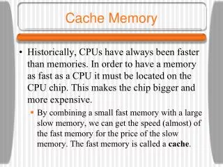

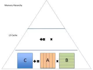


More Related