Download
1 / 33
380 likes | 602 Vues
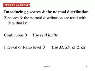
Introducing z -scores & the normal distribution Z-scores & the normal distribution are used with data that is: Continuous Use real limits Interval or Ratio level Use M, SS, , & 2. Frequency distributions & relative frequencies: X = levels or values of the variable.

E N D
Introducing z-scores & the normal distribution • Z-scores & the normal distribution are used with data that is: • ContinuousUse real limits • Interval or Ratio levelUse M, SS, , & 2 Statistics 1
Frequency distributions & relative frequencies: • X = levels or values of the variable. • f = observed data. • relative f = f/n. • Relative frequency: the proportion of observations in a given X interval. • .36 or 36% of the observations are in the X=3 interval (2.5-3.5). Statistics 1
Relative frequency: the probability of observingX in a given interval. • p(3) = .36 and p(2.5<X<3.5)=.36 • Probability of observing an X value = its relative frequency. • Probability of observing an X above/below a particular score = the sum of the probabilities above/below the interval that contains X. Statistics 1
Normal Distributions • Family of symmetrical, unimodal distributions with different & ². • Describe many of the variables of psychological interest. • IQ is a normally distributed variable with =100 & =15 • Height is a normally distributed variable with =68’’ & =6’’ • Area under the curve corresponds to proportion/probability. Statistics 1
Any normal distribution can be transformed into the unit normal distribution. • Values range from - ∞ to + ∞ =0 & =1 • The z-score transformation is used to turn distributions of raw scores into standardized scores or z-scores. • Used to estimate probabilities of outcomes & set critical values. Statistics 1
When the z-score transformation is used with a normally distributed set of scores, you get the unit normal distribution. • Each raw score has been transformed into a z-score using this formula: Statistics 1
More about z-scores • X is the raw score of interest • is the mean of the raw score population • is the standard deviation of the raw scores • Z-scores express the distance between the observation & the mean in standard deviation units. • If the observation is 1 standard deviation above the mean, z = +1. • For SAT scores, with =500 & =100 • If raw SAT score=400, z=____ • Hint, 400 is 1 standard deviation below the mean. Statistics 1
More about z-scores • X is the raw score of interest • is the mean of the raw score population • is the standard deviation of the raw scores • Z-scores express the distance between the observation & the mean in standard deviation units. • If the observation is 1 standard deviation above the mean, z = +1. • For SAT scores, with =500 & =100 • If raw SAT score=400, z=____ • Hint, 400 is 1 standard deviation below the mean. Statistics 1
If raw SAT score=650, z=____ Statistics 1
If raw SAT score=650, z=____ • indicates direction above or below the mean. • Absolute value indicates distance from the mean. • The mean has a z-score of 0. Statistics 1
Z-scores allow us to make statements about the relative location of a score in a distribution. • For distribution (a), a test score of 76 is higher than most of the other scores: • For distribution (b), a test score of 76 is only slightly above the mean: Statistics 1
Z-scores allow us to make comparisons between scores from different distributions. • Which score is more impressive: an IQ=130 or an SAT=650? Statistics 1
Z-scores allow us to make comparisons between scores from different distributions. • Which score is more impressive: an IQ=130 or an SAT=650? • IQ=130 (z = +2) is more impressive than an SAT=650 (z = +1.5). Statistics 1
When you transform an entire distribution into z-scores, you have z-score distribution or a standardized distribution. • with =0 & =1 • & the same shape as the original distribution • Converting frequency distribution (a) to a z-score distribution (b) has not changed the shape of the distribution. Statistics 1
If the raw score distribution is normal, standardization produces the unit normal distribution. • For the normal distribution, the relative frequencies/ probabilities/ proportions of the area under the curve marked by z-scores are known. Statistics 1
Mean = 3, z = 0. Statistics 1
34.13% of the normal distribution lies between the mean & a z-score of +1. • 2.28% of the normal distribution lies below a z-score of -2. Statistics 1
z-scores & the unit normal distribution • We will use the unit normal distribution to find probabilities associated with observations & to set critical values. • .025 of the unit normal distribution lies above z = +1.96; • .025 of the unit normal distribution lies below z = -1.96. Statistics 1
The unit normal table (B1) lists proportions of the normal distribution for each z-score value. • Proportions under the curve are relative frequencies/probabilities. Statistics 1
Introduction to probability: The binomial • Descriptive statistics: summarize, organize, & simplify data. • Inferential statistics: use samples to draw conclusions about the population. • If sample is typical of what we would expect, conclude the sample comes from the specified population. • If sample is very unusual or improbable, conclude the sample does NOT come from the specified population. • This logic requires us to quantify 2 things: • Our expectations about the population & • What we mean by improbable or unusual. Statistics 1
Observe 6 rats in a Y maze: 5 turn right, 1 turns left. • If chance alone is operating, • 50% of the rats should turn right. • p(right turn)=.5 • If chance alone is operating, • 3 rats should turn right. • Xe=p(right turn)*n= .5 * 6 = 3 Statistics 1
Have we observed anything unusual? • Our expectation is what we think should happen based on what we know about the population parameter, p(turning right); Xe=3. • Our observation is what actually happened with our sample; Xo=5. • To specify our expectation (Xe), we needed to know sample size (n) & the parameter, p(turning right). • If 5 rats turn right when we only expect 3, is this evidence that something unusual is going on? Statistics 1
We also need some criterion for deciding how different Xo has to be from Xe before we can conclude our observation was unusual. • “Unusual” means they do NOT come from the population of rats who are equally likely to turn left or right. • How extreme must Xo be for us to conclude that these rats come from some other population, where p(turning right) ≠.5? • Inferential statistics uses probability to set precise criteria for deciding whether or not a sample is likely to have come from a given population. • The binomial distribution is used to calculate probabilities for observations of nominal data with 2 categories. Statistics 1
Definitions & notation • Xe: the # of events expected to display the characteristic of interest. • Xo: the # events that actually display the characteristic of interest. • X: a possible value of Xo. • Null hypothesis or Ho: specifies expectations as population parameters. • n: the # of events (people, coin flips, items, trials, etc…) observed. • Probability: likelihood of observing a particular event class. • P(A): probability of observing an outcome or characteristic belonging to event class A—the one you’re interested in. • Q(B): probability of observing the only other possible outcome or characteristic, belonging to event class B—the “other one.” • Note that P+Q=1.00. Statistics 1
Parameters for the binomial: P & Q • To know what is expected in the population, we must know the parameters; for binomial these are P. & Q. • How do we know what the population parameters are? • Prior knowledge • 90% of people are right handed, so P(right handed)=.90 • Definition of the situation/chance • Rats could only turn left or right, so P(right turn)=.50 • For binomial data, Ho specifies the proportion of the population that belongs to the event class of interest. • Ho: P(right handed)=.90 Ho: P(right turn)=.50 • Why not just write Ho in terms of Xe instead of P & Q? • Xe changes as n changes, but P & Q apply to all possible n’s. Statistics 1
Assumptions for using the binomial • Any statistical test is only appropriate when the sample data meet certain requirements. For the binomial, these are: • Random sampling • Every member of the population has an • EQUAL chance of being selected. • p(selection) = 1/ N • If more than one member is selected, there must be a constant probability for each and every selection. • p(selection) always = 1/ N, never 1/N-1, 1/N-2… • Use sampling with replacement for finite populations Statistics 1
Independence of observations • The probability of an element being in the sample does NOT depend on any other element's inclusion. • Event classes must be mutually exclusive & exhaustive • Mutually exclusive: no elementary element can be a member of both event classes. • Exhaustive: every element drawn can be categorized as one or the other event class. Statistics 1
Rules for working with binomial probabilities • Additive rule/“OR rule”: • To calculate the probability of selecting one event class OR the other, ADD the probabilities together. • P(A OR B)= P(A) + P(B)-P(A & B together) • For binomial data, A & B can never occur together, so P(A & B together) always = 0. • For the sample of 6 rats in the Y-maze, what is the probability that the first animal will turn right OR turn left? • p(right turn by rat # 1) = .5 • p(left turn by rat # 1) = .5 • p (right OR left turn by rat # 1) = .5 +.5-0=1.0 Statistics 1
Multiplicative rule/ “AND rule”: • To calculate the probability of selecting a particular sequence of event classes, MULTIPLY the probabilities together. • P(A & B) = P(A)*P(B) • For the sample of 6 rats in the Y-maze, what is the probability that the first animal & the second animal will both turn right? • p(right turn by rat # 1) = .5 • p (right turn by rat # 2) = .5 • p (right turn by rat # 1 AND rat #2) = .5x.5=.25 • Notice that when the probabilities multiplied together are the same, you can summarize this using an exponent. • p (right turn by rats # 1, #2 & #3) = .53= Statistics 1
We can use this observation to calculate the probability of any particular sequence containing X # of observations of interest: • P(any sequence with a given X)= pXqn-X • X= # of observations of interest, n= # of events or trials • p= probability of observing an X on any 1 trial, • q= probability of observing a “not X” on any 1 trial • We will use both the “AND rule” & the “OR rule” to specify the exact probability of observing any given X. • Then we can decide whether an observation is “unusual.” • The exact probability of a given X will depend on: • The probability of getting any sequence that contains the X & • The # of different sequences that contain the X. Statistics 1
Calculating the probability of a particular sequence • Imagine a multiple choice test with 4 questions where each question has 5 options (a, b, c, d, or e). • We are interested in correct answers. • We want to compare our observations to what we would expect based on chance / “guessing.” • P(any sequence with a given X)=pXqn-X • n= # of events or trials = 4 • p(correct on any 1 question)=1/5=.20 • q(incorrect on any 1 question)=4/5=.80 • X= # of correct answers • The probability of observing a sequence containing X =2 correct answers is: • .22 X .82 = .0256 Statistics 1
This is the probability of any sequence containing 2 correct answers without regard to order. • Different combinations of C's (corrects) and I's (incorrects) can give us a total of X=2. • For example: • p(CCII)=.2 X .2 X .8 X.8 = .0256. • p(CICI)=.2 X .8 X .2 X .8 = .0256. • All sequences with X=2, for n=4 & p=.20 have the same probability, .0256. Statistics 1
Using the formula for combinations to calculate how many different sequences contain a particular XO • The formula pXqn-X gives you the probability of ANY sequence with a given X. • You still need to know how many different sequences or combinations of n elements will give you that same Xo. • For n = 4 & X =2, there are 6 combinations of "Cs" and "I's" which would give us an Xo =2 correct answers. • 1) CCII 3) IICC 5) ICCI • 2) CICI 4) ICIC 6) CIIC Statistics 1