Probability and statistics
Probability and statistics. Dr. K.W. Chow Mechanical Engineering. Contents. Review of basic concepts: - permutations - combinations - random variables - conditional probability Binomial distribution. Contents. Poisson distribution Normal distribution Hypothesis testing. Basics.


Probability and statistics
E N D
Presentation Transcript
Probability and statistics Dr. K.W. Chow Mechanical Engineering
Contents • Review of basic concepts: - permutations - combinations - random variables - conditional probability • Binomial distribution
Contents • Poisson distribution • Normal distribution • Hypothesis testing
Basics • Principle of counting: There are mndifferent combinations of marriage (i.e. for each lady, there are n possible marriage combinations, thus mn) m women n men A B
Basics • Permutation (order important ): Form a 3-digit number from (1, 2,…9) • Combination (order unimportant ): Mary marries John = John marries Mary
Permutations • Permutations of n things taken r at a time (assuming no repetitions): • For the first slot / vacancy, there are n choices. • For the second slot / vacancy, there are (n –1) choices. • Thus there are n(n– 1)…(n–r + 1) = n!/(n–r)! ways.
Combinations • Combinations of n things taken r at a time (assuming order unimportant): • Permutations: n(n– 1)…(n–r + 1) = n!/(n–r )! ways. • Every r! combinations are equivalent to a single way. • Hence number of combinations: • n!/((n–r)! r ! )
Conditional Probability • The probability that an event B occurs, given that another event A has happened. • Definition: • Note that when B and A are independent, then
Random variables • (Intuitive) Random variables are quantities whose values are random and to which a probability distribution is assigned. • Either discrete or continuous.
Random variables • Example of random variables: Outcome of rolling a fair die
Random variables • All possible outcomes belong to the set: • Outcome is ‘random’. • Probabilities of every outcome are the same, i.e. the outcomes follow the uniform distribution. • Hence the outcomes are random variables.
Random variables • (Rigorous definition) Random variable is a MAPPING from elements of the sample space to a set of real numbers (or an interval on the real line). • e.g. for a fair die – mapping from {1, 2,3,4,5,6} to 1/6.
Probability density function • In physics, mass of an object is the integral of density over the volume of that object: • Probability density function (pdf) f(x)is defined such that the probability of a random variable X occurring between a and b is equal to the integral of f between a and b.
Probability density function Defining properties: • Probability density function is non-negative. • The integral over the whole sample space (e.g. the whole real axis) must be unity.
Probability density function • The probability is not defined at single point, it does not make sense to say what is the chance of x = 1.23 for a continuous random variable, as that chance is zero (infinitely many points).
Probability density function • For discrete random variables, the probability at a point is equal to the probability density function evaluated at that point: • Probability between two points (inclusive):
Cumulative density function • Cumulative density function (cdf) F is related to pdf by: • Note: the lower limit is the smallest value that ηcan take, not necessarily
Cumulative density function • For discrete random variables: • cdf’s for discrete random variables are discontinuous
Cumulative density function cdf of a discrete random variable cdf of a continuous random variable
Expectation and variance of random variables • Expectation (or mean): Integral or sum of the probability of an outcome multiplied by that outcome. • For continuous variables, the “probability” of X falling in the interval (x, x+dx) is:
Expectation and variance of random variables • The expectation is: • The integral is taken over the whole sample space. • Not all distributions have expectation, since the integral may not exist, e.g. the Cauchy distribution.
Expectation and variance of random variables • For discrete variables, the “probability” of an outcome is: • The expectation is:
Expectation and variance of random variables • Expectation represents the average amount one "expects" as the outcome of the random trial when identical experiments are repeated many times.
Expectation and variance of random variables • Example: Expectation of rolling a fair die: • Note that this “expected value” is never achieved !!
Expectation and variance of random variables • Standard deviation : a measure of how a distribution is spread out relative to the mean. • Definition:
Expectation and variance of random variables • Variance is defined as the square of standard deviation:
Binomial distribution • Bernoulli experiment: outcome is either success or fail. • The number of successes in n independent Bernoulli experiments are governed by the Binomial distribution. • This is a distribution with discrete random variables.
Binomial distribution • Suppose we perform an experiment 4 times. What is the chance of getting three successes? (Chance for success = p, chance for failure = q, p + q = 1).
Binomial distribution • Scenario: • p, p, p, q • p, p, q, p • p, q, p, p • q, p, p, p • There are 4C3 ways of placing the failure case.
Binomial distribution • Thus the chance is 4 p3 q. • For a simpler case – getting 2 heads in throwing a fair coin 3 times: • H, H, T; • H, T, H; • T, H, H.
Binomial distribution • Example: chance of getting exactly 2 heads when a fair coin is tossed 3 times is:
Binomial distribution • The probability density function for r successes in a fixed number (n ) trials is: • (r = 0, 1, 2…n) where r is the number of successes, and p is the probability of success of each trial.
Binomial distribution • Expectation: • Variance:
Binomial distribution • Methods to derive the formula E(X) = np for the binomial distribution: (1) Direct argument: Gain of p at each trial. Hence total gain of np in n trials. (2) Direct summation of series. (3) Differentiate the series expansion of the ‘binomial theorem’.
Binomial distribution The probability density function
Binomial distribution The cumulative density function
Poisson distribution • Poisson distribution is a special limiting case of the binomial distribution by taking: while keeping the product npfinite. • The probability density function is:
Poisson distribution • Expectation of the Poisson distribution: • Variance of the Poisson distribution:
The Poisson distribution • Physical meaning: a large number of trials (n going to infinity), and the probability of the event occurring by itself is pretty small (p approaching zero). • BUT (!!) the combined effect is finite (np being finite).
The Poisson distribution • Examples: • (a) The number of incorrectly dialed telephone calls if you have to dial a huge number of calls. • (b) Number of misprints in a book. • (c) Number of accidents on a highway in a given period of time.
Poisson distribution The probability density function (usually shows a single maximum).
Poisson distribution The cumulative density function (must start from zero and end up in one)
Normal distribution • The normal distribution for a continuous random variable is a bell-shaped curve with a maximum at the mean value. It is a special limit of the binomial distribution when the number of data points is large (i.e. ‘n going to infinity’ but without special conditions on p).
Normal distribution • As such the normal distribution is applicable to many physical problems and phenomena. • The ‘Central Limit Theorem’ in the theory of probability asserts the usefulness of the normal distribution.
Normal distribution • The probability density function: where
Normal distribution • The curve is symmetric about The probability density function
Normal distribution • For small standard deviation, the curve is tall, sharply peaked and narrow. • For large standard deviation, the curve is short and widely spread out. • (As the area under the curve must sum up to one to be a probability density function).
Normal distribution The cumulative density function
Normal distribution • Cumulative density function or probability of a normally distributed random variable falling within the interval (a, b): • Values of the above integral can be found from standard tables.
Simple tutorial examples for the normal distribution It is obviously not possible to tabulate the normal distribution pdf for all values of mean and standard deviation. In practice, we reduce, by simple ‘scaling arguments’, every normal distribution problem to one with mean zero and standard deviation. (Notation: N(μ, σ2))