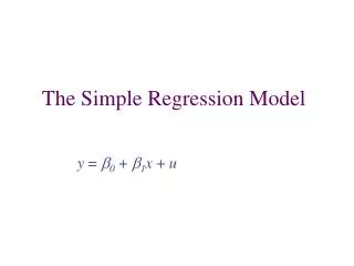
I. Introduction: Simple Linear Regression
I. Introduction: Simple Linear Regression. As discussed last semester, what are the basic differences between correlation & regression? What vulnerabilities do correlation & regression share in common? What are the conceptual challenges regarding causality?.


I. Introduction: Simple Linear Regression
E N D
Presentation Transcript
I. Introduction: Simple Linear Regression
As discussed last semester, what are the basic differences between correlation & regression? • What vulnerabilities do correlation & regression share in common? • What are the conceptual challenges regarding causality?
Linear regression is a statistical method for examining how an outcome variable y depends on one or more explanatory variables x. • E.g., what is the relationship of the per capita earnings of households to their numbers of members & their members’ ages, years of higher education, race-ethnicity, gender & employment statuses?
What is the relationship of the fertility rates of countries to their levels of GDP per capita, urbanization, education, & so on? • Linear regression is used extensively in the social, policy, & other sciences.
Multiple regression—i.e. linear regression with more than one explanatory variable—makes it possible to: • Combine many explanatory variables for optimal understanding &/or prediction; & • Examine the unique contribution of each explanatory variable, holding the levels of the other variables constant.
Hence, multiple regression enables us to perform, in a setting of observational research, a rough approximation to experimental analysis. • Why, though, is experimental control better than statistical control? • So, to some degree multiple regression enables us to isolate the independent relationships of particular explanatory variables with an outcome variable.
So, concerning the relationship of the per capita earnings of households to their numbers of members & their members’ ages, years of education, race-ethnicity, gender & employment statuses: • What is the independent effect of years of education on per capita household earnings, holding the other variables constant?
Regression is linearbecause it’s based on a linear (i.e. straight line) equation. • E.g., for every one-year increase in a family member’s higher education (an explanatory variable), household per capita earnings increase by $3127 on average, holding the other variables fixed.
But such a statistical finding raises questions: e.g., is a year of college equivalent to a year of graduate school with regard to household earnings? • We’ll see that multiple regression can accommodate nonlinear as well as linear y/x relationships. • And again, always question whether the relationship is causal.
Before proceeding, let’s do a brief review of basic statistics. • A variable is a feature that differs from one observation (i.e. individual or subject) to another.
What are the basic kinds of variables? • How do we describe them in, first, univariate terms, & second, bivariate terms? • Why do we need to describe them both graphically & numerically?
What’s the fundamental problem with the mean as a measure of central tendency & standard deviation as a measure of spread? When should we use them? • Despite their problems, why are the mean & standard deviation used so commonly?
What’s a density curve? A normal distribution? What statistics describe a normal distribution? Why is it important? • What’s a standard normal distribution? What does it mean to standardize a variable, & how is it done? • Are all symmetric distributions normal?
What’s a population? A sample? What’s a parameter? A statistic? What are the two basic probability problems of samples, & how most basically do we try to mitigate them? • Why is a sample mean typically used to estimate a parameter? What’s an expected value?
What’s sampling variability? A sampling distribution? A population distribution? • What’s the sampling distribution of a sample mean? The law of large numbers? The central limit theorem? • Why’s the central limit theorem crucial to inferential statistics?
What’s the difference between a standard deviation & a standard error? How do their formulas differ? • What’s the difference between the z- & t-distributions? Why do we typically use the latter?
What’s a confidence interval? What’s its purpose? Its premises, formula, interpretation, & problems? How do we make it narrower? • What’s a hypothesis test? What’s its purpose? Its premise & general formula? How is it stated? What’s its interpretation?
What are the typical standards for judging statistical significance? To what extent are they defensible or not? • What’s the difference between statistical & practical significance?
What are Type I & Type II errors? What is the Bonferroni (or other such) adjustment? • What are the possible reasons for a finding of statistical insignificance?
True or false, & why: • Large samples are bad. • To obtain roughly equal variability, we must take a much bigger sample in a big city than in a small city. • You have data for an entire population. Next step: construct confidence intervals & conduct hypothesis tests for the variables. Source: Freedman et al., Statistics.
(true-false continued) • To fulfill the statistical assumptions of correlation or regression, what definitively matters for each variable is that its univariate distribution is linear & normal. • __________________________
Define the following: • Association • Causation • Lurking variables • Simpson’s Paradox • Spurious non-association • Ecological correlation
Restricted-range data • Non-sampling errors • _________________________
Regarding variables, ask: • How they are defined & measured? • In what ways are their definition & measurement valid or not? • & what are the implications of the above for the social construction of reality? • See King et al., Designing Social Inquiry; & Ragin, Constructing Social Research.
Remember the following, overarching principles concerning statistics & social/policy research from last semester’s course: (1) Anecdotal versus systematic evidence (including the importance of theories in guiding research). (2) Social construction of reality.
(3) Experimental versus observational evidence. (4) Beware of lurking variables. (5) Variability is everywhere. (6) All conclusions are uncertain.
Recall the relative strengths & weaknesses of large-n, multivariate quantitative research versus small-n, comparative research & case-study research. • “Not everything worthwhile can be measured, and not everything measured is worthwhile.” Albert Einstein
Finally, here are some more or less equivalent terms for variables: • e.g., dependent, outcome, response, criterion, left-hand side • e.g., independent, explanatory, predictor, regressor, control, right-hand side • __________________________
The dean of students wants to predict the grades of all students at the end of their freshman year. After taking a random sample, she could use the following equation:
Since the dean doesn’t know the value of the random error for a particular student, this equation could be reduced to using the sample mean of freshman GPA to estimate a particular student’s GPA: That is, a student’s predicted y (i.e. yhat) is estimated as equal to the sample mean of y.
But what does that mini-model overlook? • That a more accurate model—& thus more precise predictions—can be obtained by using explanatory variables (e.g., SAT score, major, hours of study, gender, social class, race-ethnicity) to estimate freshman GPA.
Here we see a major advantage of regression versus correlation: regression permits y/x directionality* (including multiple explanatory variables). • In addition, regression coefficients are expressed in the units in which the variables are measured. • * Recall from last semester: What are the ‘two regression lines’? What questions are raised about causality?
We use a six-step procedure to create a regression model (as defined in a moment): • Hypothesize the form of the model for E(y). • Collect the sample data on outcome variable y & one more more explanatory variables x: random sample, data on all the regression variables are collected for the same subjects. • Use the sample data to estimate unknown parameters in the model.
(4) Specify the probability distribution of the random error term (i.e. the variability in the predicted values of outcome variable y), & estimate any unknown parameters of this distribution. (5) Statistically check the usefulness of the model. (6) When satisfied that the model is useful, use it for prediction, estimation, & so on.
We’ll be following this six-step procedure for building regression models throughout the semester. • Our emphasis, then, will be on how to build useful models: i.e. useful sets of explanatory variables x’s and forms of their relationship to outcome variable y.
“A model is a simplification of, and approximation to, some aspect of the world. Models are never literally ‘true’ or ‘false,’ although good models abstract only the ‘right’ features of the reality they represent” (King et al., Designing Social Inquiry, page 49). • Models both reflect & shape the social construction of reality.
We’ll focus, then, on modeling: trying to describe how sets of explanatory variables x’s are related to outcome variable y. • Integral to this focus will be an emphasis on the interconnections of theory & empirical research (including questions of causality).
We’ll be thinking about how theory informs empirical research, & vice versa. • See King et al., Designing Social Inquiry; Ragin, Constructing Social Research; McClendon, Multiple Regression and Causal Analysis; Berk, Regression: A Constructive Critique.
“A social science theory is a reasoned and precise speculation about the answer to a research question, including a statement about why the proposed answer is correct.” • “Theories usually imply several or more specific descriptive or causal hypotheses” (King et al., page 19). • And to repeat: A model is “a simplification of, and approximation to, some aspect of reality” (King et al., page 49).
One more item before we delve into regression analysis: Regarding graphic assessment of the variables, keep the following points in mind: • Use graphs to check distributions & outliers before describing or estimating variables & models; & after estimating models as well.
The univariate distributions of the variables for regression analysis need not be normal! • But the usual caveats concerning extreme outliers must be heeded. • It’s not the univariate graphs but the y/x bivariate scatterplots that provide the key evidence on these concerns.
Even so, let’s anticipate a fundamental feature of multiple regression: • The characteristics of bivariate scatterplots & correlations do not necessarily predict whether explanatory variables will be significant or not in a multiple regression model.
Moreover, bivariate relationships don’t necessarily indicate whether a Y/X relationship will be positive or negative within a multivariate framework.
This is because multiple regression expresses the joint, linear effects of a set of explanatory variables on an outcome variable. • See Agresti/Finlay, chapter 10; and McClendon, chapter 1 (and other chapters).
Let’s start our examination of regression analysis, however, with a simple (i.e. one explanatory variable) regression model:
. su science math . corr science math . scatter science math||qfit science math