Download
1 / 106
1.07k likes | 1.95k Vues
Chapter 4: Simple or Bivariate Regression. Terms Dependant variable (LHS) the series we are trying to estimate Independent variable (RHS) the data we are using to estimate the LHS. The line and the regression line. Y = f(X)…there is assumed to be a relationship between X and Y.

E N D
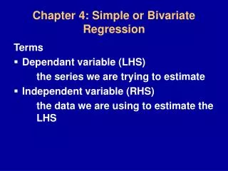
Chapter 4: Simple or Bivariate Regression Terms • Dependant variable (LHS) the series we are trying to estimate • Independent variable (RHS) the data we are using to estimate the LHS
The line and the regression line • Y = f(X)…there is assumed to be a relationship between X and Y. • Y = Mx + b Because the line we are looking for is an estimate of the population, and not every observation falls on the estimate of the line we have error (e). • Y = b0+ b1X1+e
What isb • b0represents the intercept term. • b1 represents the slope of the estimated regression line. This term (b1) can be interpreted as the rate of change in Y with per unit change in X…just like a simple line eq.
Population vs Sample • Y = b0 + b1X1 + e • = b0 + b1X1 + e Population (We don’t often have this data) Sample (We usually have this) Y - = e (a.k.a. error or the residuals)
Residuals another way • Residuals can also be constructed by solving for e in the regression equation. • e = Y - b0 – b1*X
The goal of Ordinary Least-Squares Regression (the type we are going to use) • Minimize the sum of squared residuals. • We could calculate the regression line and the residuals by hand….but, we ain’t gonna.
First step: ALWAYS, look at your data • Plot it against time, or • Plot it against your dependent variable. • Why?...because dissimilar data can potentially generate very similar summary statistics…pictures help discern the differences…
Dissimilar data with similar stats X’s have the same mean and St. Dev. Y’s have the same mean and St. Dev. From this we might conclude that each of the data sets are identical, but we’d be wrong
What do they look like? Although, they result in the same OLS regression, they are very different.
Forecasting: Simple Linear Trend Disposable Personal Income (DPI) • It’s sometimes reasonable to make a forecast on the basis of just a linear trend, where Y is just assumed to be a function of (T) or time. • The regression looks like the following: • Where Y(hat) is the series you want to estimate. In this case, it’s DPI.
To forecast with Simple OLS in ForecastX… • You need to construct an index of T For this data set, there are 144 months. Index goes from 1-144 T The Data
Jan 1993: DPI1= 4588.58 + 27.93 (1) = 4616.51 Feb 1993: DPI2= 4588.58 + 27.93 (2) =4644.44 . . . Dec 2004: DPI144= 4588.58 + 27.93 (144) =8610.50 Dec 2004: DPI145= 4588.58 + 27.93 (145) =8638.43 And, so on… To forecast, we just need the index for the month (T)
Output Hypothesis test for slope = 0 and intercept = 0…What does it say
Sampling distribution of Do we reject that the slope and intercept are each equal to 0?! 138.95 297.80 Reject H0 Reject H0 Do Not Reject H0 t 0 2.045 -2.045
Just to note… • In the previous model, the only thing we are using to predict DPI is the progression of time. • There are many more things that have the potential of increasing or decreasing DPI. • We don’t account for anything else…yet.
The benefits of regression • The true benefits of regression models is in its ability to examine cause and effect. • In trend models (everything we’ve seen until now), we are depending on observed patterns of past values to predict future values. • In a Causal model, we are hypothesizing a relationship between the dependent variable (the variable we are interested in predicting) and one or more independent variables (the data we use to predict).
Back to Jewelry • There many things that might influence the total monthly sales of jewelry…things like • - # Weddings • - # Anniversaries • - Advertising expenditures, and • - DPI • Since this is bivariate regression, for now we will focus on DPI as the sole independent variable used to predict jewelry sales.
Let’s Look at the jewelry sales data plotted against DPI Christmas Othermonths The big differences in sales during the Dec. months will make it hard to estimate with a bivariate regression. We will use both the unadjusted and the seasonally adjusted series to see the difference in model accuracy.
Jewelry Example • Our dependent (Y) variable is monthly jewelry sales • unadjusted in the first example • seasonally adjusted in the second example • Our only independent variable (X) is DPI, so the models we are going to estimate are: • JS= b0 + b1*(DPI) + e • SAJS= b0 + b1*(DPI) + e
Things to consider with ANY regression • Do the signs on the b’s make sense? • Your expectation should have SOME logical basis. • If the sign is not what is expected, your regression may be: • Underspecified-move on to multiple regression. • Misspecified-consider other RHS variables that might provide a better measure.
Consider the Jewelry Example • Do we get the right sign? i.e., what’s the relationship between DPI and sales? • What is a normal good? • What kind of good is jewelry, normal or inferior? • What would be the expected sign if we were looking at a good we though was and inferior good?
Things to consider with ANY regression • If you DO get the expected signs, are the effects statistically significant? • Do the t-stats indicate a strong relationship? • Can you reject the null that the relationship (slope) is 0?
Things to consider with ANY regression • Are the effects economically significant • Even with statistically significant results, a very small slope indicates a very large change in the RHS variable is necessary to get any change in the LHS. • There is no hard & fast rule here. It requires judgment.
Consider the Jewelry Example • In the jewelry example, it takes a $250 million (or $.25 billion) dollar increase in DPI to increase (adjusted) jewelry sales by $1 million. Is this a lot or a little slope? Let’s think of it a little differently… • T his would be roughly a $1 increase in (adjusted) jewelry sales with a $250 increase in personal disposable income. • Does this pass the “sniff test?”
Things to consider with ANY regression • Does the regression explain much? • In linear regressions, the fraction of the “variance” in the dependent variable “explained” by the independent variable is measured by the R-squared (A.K.A. the Coefficient of Variation). Trend: R-sq = .9933 Causal (w/season): R-sq = .0845 Causal (w/o season): R-sq = .8641 Although the causal model explains less of the variance, we now have some evidence that sales are related to DPI.
Another thing to consider about the first model w/seasonality in it • The first model was poorly specified when we were using the series with seasonality in it. • The de-seasonalized data provides better fit in the simple regression. • …why? • Well, income is obviously related to sales, but so is the month of the year (e.g., Dec), so we need to adjust or account. • Adjust for seasonality (use a more appropriate RHS var) , or • Account for it in the model (move to multi-var and include the season in the regression…to be covered next chapt.)
Question • Why would we want to forecast Jewelry sales based on a series like DPI? • DPI is very close to a linear trend…we have a good idea what it might look like a several periods from now.
Other examples of simple regression models:Cross section (all in the same time) • Car mileage as a function of engine size • What do we expect this relationship to be on average? • Body weight as a function of height • What do we expect this relationship to be on average? • Income as a function of educational attainment • What do we expect this relationship to be on average?
Assumptions of the OLS regression • One assumption of the OLS model is that the error terms DON’T have any regular patters. First off, this means… • Errors are independantly distributed • And, they are normally distributed • They have a mean of 0 • They have a constant variance
Errors are independantly distributed Errors might not be independantly distributed if we have Serial Correlation (or Autocorrelation) • Serial correlation occurs when one period’s error is related to another period’s error • You can have both positive and negative serial correlation
Negative Serial Correlation • Negative serial correlation occurs when positive errors are followed by negative errors (or vice versa) Y X
Positive Serial Correlation • Positive serial correlation occurs when positive errors tend to be followed by positive errors Y X
What does Serial Correlation Cause? • The estimates for b are unbiased, but the errors are underestimated…this means our t-stats are overstated. • If our t-stats are overstated, then it’s possible we THINK we have a significant effect for b, when we really don’t. • Additionally, R-squared and F-stat are both unreliable.
Durbin-Watson Statistic • The Durbin-Watson Statistic is used to test for the existence of serial correlation. Sum of Sq Errors The Durbin-Watson Statistic ranges from 0 to 4.
Evaluation of the DW Statistic The rule of thumb: If it’s near 2 (i.e., from 1.5 - 2.5) there is no evidence of serial correlation present. For more precise evaluation you have to calculate and compare 5 inequalities and determine which of the 5 is true.
# of RHS vars Lower and Upper DW
Evaluation of the DW Statistic Evaluate (Choose True Region) 4 > DW > (4-DWL) T/F A • (4-DWL) > DW > (4-DWU) T/F B • (4-DWU) > DW > DWU T/F C • DWU > DW > DWL T/F D • DWL > DW > 0 T/F E Negative serial correlation Positive serial correlation Indeterminate or no observed serial correlation
For Example • Suppose we get a DW of 0.21 with a 36 observations… From the table: DWL = 1.41 DWU= 1.52 • The rest is just filling in and evaluating. 4 > 0.21 > (4 - 1.41) T/F A (4 - 1.41) > 0.21 > (4 -1.52) T/F B (4-1.52) > 0.21 > 1.52 T/F C 1.52 > 0.21 > 1.41 T/F D 1.41 > 0.21 > 0 T/F E
Errors are Normally Distributed Each observation’s error is normally distributed around the estimated regression line. OLS Regression Line Y Error can be +/-, but they are grouped around the regression line. X
When might errors be distributed some other way??? • One example would be a dependant variable that’s like 0/1 or similar (discrete and/or limited). • Employed/Unemployed • Full-time/Part-time • =1 if above a certain value, =0 if not.