Bivariate Correlation & Regression
Bivariate Correlation & Regression. correlation vs. prediction research Interpreting scatterplots and correlations quantitative vs. binary predictor variables prediction and relationship strength interpreting regression formulas quantitative vs. binary predictor variables

Bivariate Correlation & Regression
E N D
Presentation Transcript
Bivariate Correlation & Regression • correlation vs. prediction research • Interpreting scatterplots and correlations • quantitative vs. binary predictor variables • prediction and relationship strength • interpreting regression formulas • quantitative vs. binary predictor variables • raw score vs. standardized formulas • selecting the correct regression model • regression as linear transformation (how it works!) • process of a prediction study
Correlation Studies and Prediction Studies • Correlation research (95%) • purpose is to identify the direction and strength of linear relationship between two quantitative variables • usually theoretical hypothesis-testing interests • Prediction research (5%) • purpose is to take advantage of linear relationships between quantitative variables to create (linear) models to predict values of hard-to-obtain variables from values of available variables • use the predicted values to make decisions about people (admissions, treatment availability, etc.) • However, to fully understand important things about the correlation models requires a good understanding of the regression model upon which prediction is based...
A scatterplota graphical depiction of the relationship between two quantitative (or binary) variables • each participant’s x & y values depicted as a point in x-y space • Pearson’s correlation coefficient (r value) summarizes the direction and strength of the linear relationship between two quantitative variables into a single number (range from -1.00 to 1.00) • you should always examine the scatterplot before considering the correlation between two variable • NHST can be applied to test if the correlation in the sample is sufficiently large to reject H0: of no linear relationship between the variables in the population • A linear regression formula allows us to take advantage of this relationship to estimate or predict the value of one variable (the criterion) from the other (the predictor). • prediction should only be applied if the relationship between the variables is “linear” and “substantial”
Example of a “scatterplot” Puppy Age (x)Eats (y) Sam Ding Ralf Pit Seff … Toby 5 4 3 2 1 0 8 20 12 4 24 .. 16 2 4 2 1 4 .. 3 Amount Puppy Eats (pounds) 4 8 12 16 20 24 Age of Puppy (weeks)
We can use correlation to examine the relationship between a quantitative predictor variable and a quantitative criterion variable. Y Y Y strong + weak + +1.00 X X X A positive r tells us those higher X values tend to have higher Y values Y Y Y strong - weak - .00 X X X A negative r tells us those with lower X values tend to have higher Y values A nonsignificant r tells us there is no linear relationship between X & Y
We can also use correlation to examine the relationship between a binary predictor variable and a quantitative criterion variable. Y Y Y strong + weak + +1.00 grp 1 grp 2 grp 1 grp 2 grp 1 grp 2 A positive r tells us the group with the higher X code as the higher mean Y Y Y Y strong - weak - .00 grp 1 grp 2 grp 1 grp 2 grp 1 grp 2 A negative r tells us the group with the lower X code as the higher mean Y A nonsignificant r tells us the groups have “equivalent” means on Y
Interpret each of the following (significance, strength & direction) For age & social skills: r = .25, p = .043. For practice and performance errors: r = -.52, p = .015 For age and performance: r = -.33, p = .231 For gender (m=1, f=2) and social skills: r = .14, p = .004 For gender (m=1, f=2) and performance: r = -.31, p = .029 For gender (m=1, f=2) and practice: r = .11, p = .098 Sig – medium – positive Older adolescents tend to have higher social skills scores Sig – large – negative Those who practiced more tended to have fewer errors Nonsig – medium? - negative ? There is no linear relationship between age and performance Sig – small – positive Females had higher mean on social skills scores Sig – medium – negative Males had higher mean performance Nonsig – small? – positive? No mean practice difference between males & females
Extreme Non-linear relationship • r value is “misinformative” Scatterplot as correlation “sees it” actual scatterplot notice... there is an x-y relationship regression line has 0 slope & r = 0 -- no linear relationship
Moderate Non-linear relationship • r value is an underestimate of the strength of the nonlinear relationship Scatterplot as correlation “sees it” actual scatterplot notice... there is an x-y relationship regression line has non-0 slope & r ~= 0 but, the regression line not a great representation of the bivariate relationship
Linear regression for prediction... • linear regression “assumes” there is a linear relationship between the variables involved • “if two variables aren’t linearly related, then you can’t use one as the basis for a linear prediction of the other” • “a significant correlation is the minimum requirement to perform a linear regression” • a significant correlation means that bivariate prediction will work “better than chance” • a significant correlation means that bivariate prediction will work better than predicting everybody will have the mean • sometimes even a small significant correlation can lead to useful prediction
Let’s take a look at the relationship between the strength of the linear relationship and the accuracy of linear prediction. • for a given value of X • draw up to the regression line • draw over the predicted value of Y When the linear relationship is very strong, there is a narrow range of Y values for any X value, and so the Y’ “guess” will be close Y’ Y Notice that everybody with the same X score will have the same predicted Y score. There won’t be much error, though, because there isn’t much variability of the Y scores for any given X score. Criterion Predictor X X
However, when the linear relationship is very weak, there is a wide range of Y values for any X value, and so the Y’ “guess” will be less accurate, on the average. There is still some utility to the linear regression, because larger values of X still “tend to” go with larger values of Y. So the linear regression might supply useful information, even if it isn’t very precise -- depending upon what is “useful”? Y’ Criterion Predictor X Notice that everybody with the same X score will have the same predicted Y score. Now there will be lots of error, because there is a lot of variability of the Y scores for any given X score.
When there is no linear relationship, everybody has the same predicted Y score – the mean of Y. This is known as “univariate prediction” – when we don’t have a working predictor, our best guess for each individual is that they will have the mean. Y’ Criterion Predictor X X X • Some key ideas we have seen are: • everyone with a given “X” value will have the same predicted “Y” value • if there is no (statistically significant & reliable) linear relationship, then there is no basis for linear prediction • the stronger the linear relationship, the more accurate will be the linear prediction (on the average)
Predictors, predicted criterion, criterion and residuals Here are two formulas that contain “all you need to know” y’= bx+ aresidual=y-y’ y the criterion -- variable you want to use to make decisions, but “can’t get” for each participant (time, cost, ethics) x the predictor -- variable related to criterion that you will use to make an estimate of criterion value for each participant y’ the predicted criterion value -- “best guess” of each participant’s y value, based on their x value --that part of the criterion that is related to (predicted from) the predictor residual difference between criterion and predicted criterion values -- the part of the criterion not related to the predictor -- the stronger the correlation the smaller the residual (on average)
Simple regression y’ = bx + a raw score form b -- raw score regression slope or coefficient a-- regression constant or y-intercept For aquantitative predictor a = the expected value of y if x = 0 b = the expected direction and amount of change in the criterion for a 1-unit increase in the For abinary x with 0-1 coding a= the mean of y for the group with the code value = 0 b= the mean y difference between the two coded groups
standard score regression Zy’ = Zx • for a quantitative predictor tells the expected Z-score change in the criterion for a 1-Z-unit increase in that predictor, holding the values of all the other predictors constant • for a binary predictor, tells size/direction of group mean difference on criterion variable in Z-units, holding all other variable values constant • Why no “a” • The mean of Zx= 0. So, the mean of Zx= 0, which mimics the mean of Zy’ = 0 (without any correction). • Which regression model to use, raw or standardized? • depends upon the predictor data you have … • Have raw predictor scores use the raw score model • Have standardized scores use the standardized model
Let’s practice -- quantitative predictor ... #1 depression’ = (2.5 * stress) + 23 apply the formula -- patient has stress score of 10 dep’ = interpret “b” -- for each 1-unit increase in stress, depression is expected to by interpret “a” -- if a person has a stress score of “0”, their expected depression score is #2 job errors = ( -6 * interview score) + 95 apply the formula -- applicant has interview score of 10, expected number of job errors is interpret “b” -- for each 1-unit increase in intscore, errors are expected to by interpret “a” -- if a person has a interview score of “0”, their expected number of job errors is 48 increase 2.5 23 35 decrease 6 95
Let’s practice -- binary predictor ... #1 depression’=(7.5 * tx group) +15.0 code: Tx=1 Cx=0 interpret “a” -- mean of the Cx group (code=0) is interpret “b” -- the Tx group has mean than Cx so … mean of Tx group is #2 job errors = ( -2.0 * job) + 8 code: mgr=1 sales=0 the mean # job errors of the sales group is the mean difference # job errors between the groups is the mean # of job errors of the mgr group is 15 7.5 more 22.5 8 -2 6
Selecting the proper regression model (predictor & criterion) For any correlation between two variables (e.g., GRE and GPA) there are two possible regression formulas -- depending upon which is the Criterion and Predictor criterionpredictor GRE’ = b(GPA) + a GPA’ = b(GRE) + a (Note: the b and a values are NOT interchangeable between the two models) The criterion is the variable that “we want a value for but can’t have” (because “hasn’t happened yet”, cost or ethics). The predictor is the variable that “we have a value for”.
Linear regression as linear transformations: y’ = bX + a this formula is made up of two linear transformations -- bX = a multiplicative transformation that will change the standard deviation and mean of X +a = an additive transformation which will further change the mean of X A good y’ will be a “mimic” of y -- each person having a value of y’ as close as possible to their actual y value. This is accomplished by “transforming” X into Y with the mean and standard deviation of y’ as close as possible to the mean and standard deviation of Y First, the value of b is chosen to get the standard deviation of y’ as close as possible to y -- this works better or poorer depending upon the strength of the x,y linear relationship. Then, the value of a is chosen to get the mean of y’ to match the mean of Y -- this always works exactly -- mean y’ = mean Y.
Let’s consider models for predicting GRE and GPA • Each GRE scale has mean = 500 and std = 100 • GPA usually has a mean near 3.2 and std near 1.0 • say we want to predict GRE from GPA GRE’ = b(GPA) + a • we will need a very large b-value -- to transform GPA with a std of 1 into GRE’ with a std of 100 • but, say we want to predict GPA from GRE GPA’ = b(GRE) +a • we will need a very small b-value -- to transform GRE with a std of 100 into GPA’ with a std of 1 • Obviously we can’t use these formulas interchangeably -- we have to properly determine which variable is the criterion and which is the predictor and obtain and use the proper formula!!!
Conducting a Prediction Study • This is a 2-step process • Step 1 -- using the “Modeling Sample” which has values for both the predictor and criterion. • Determine that there is a significant linear relationship between the predictor and the criterion. • If there is an appreciable and significant correlation, then build the regression model (find the values of b and a) • Step 2 -- using the “Application Sample” which has values for only the predictor. • Apply the regression model, obtaining a y’ value for each member of the sample