Understanding Bivariate Methods: Correlation and Covariance in Statistical Relationships

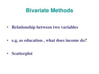
1. Bivariate Methods • Relationship between two variables • e.g, as education ­, what does income do? • Scatterplot

2. Correlation

3. Linear Correlation Source: Earickson, RJ, and Harlin, JM. 1994. Geographic Measurement and Quantitative Analysis. USA: Macmillan College Publishing Co., p. 209.

5. Wet – May 29/30 Avg. – June 26/28 Dry – August 22 Pond Branch - PG 11.25m DEM R2=0.79 R2=0.79 R2=0.71 Glyndon – LIDAR 0.5m DEM 11x11 R2=0.24 R2=0.10 R2=0.29

6. Theta-TVDI Scatterplots

7. API-TVDI Scatterplot

8. Covariance: Interpreting Scatterplots • General sense (direction and strength) • Subjective judgment • More objective approach • Extent to which variables Y and X vary together • Covariance

9. i=n S 1 (xi - x)(yi - y) Cov [X, Y] = n - 1 i=1 Covariance Formulae

10. Covariance Example

11. 2 3 4 5 1 Covariance Example

12. How Does Covariance Work? • X and Y are positively related • xi > x yi > y • xi < x yi < y • X and Y are negatively related • xi > x yi < y • xi < x  yi > y __ __ __ __ __ __ __ __

13. Interpreting Covariances • Direction & magnitude • Cov[X,Y] > 0  positive • Cov[X, Y] < 0  negative • abs(Cov[X, Y]) ↑ strength ↑ • Magnitude ~ units

14. Covariance  Correlation • Magnitude ~ units • Multiple pairs of variables  not comparable • Standardized covariance • Compare one such measure to another

15. i=n S (xi - x)(yi - y) i=1 (n - 1) sXsY r = r = i=n ZxZy S Cov [X, Y] r = sXsY i=1 (n - 1) Pearson’s product-moment correlation coefficient

16. Pearson’s Correlation Coefficient • r [–1, +1] • abs(r) ↑ strength ↑ • r cannot be interpreted proportionally • ranges for interpreting r values • 0 - 0.2 Negligible • 0.2 - 0.4 Weak • 0.4 - 0.6 Moderate • 0.6 - 0.8 Strong • 0.8 - 1.0 Very strong

17. Example • X = TVDI, Y = Soil Moisture • Cov[X, Y] = -0.017063 • SX = 0.170, SY = 0.115 • r ?

18. Pearson’s r - Assumptions • interval or ratio • Selected randomly • Linear • Joint bivariate normal distribution

19. Interpreting Correlation Coefficients • Correlation is not the same as causation! • Correlation suggests an association between variables • Both X and Y are influenced by Z

20. Interpreting Correlation Coefficients • Causative chain (i.e. X  A  B  Y) • e.g. rainfall  soil moisture  ground water  runoff • Mutual relationship • e.g., income & social status • 4. Spurious relationship • e.g., Temperature (different units) • 5. A true causal relationship (X  Y)

21. Interpreting Correlation Coefficients • A result of chance • e.g., your annual income vs. annual population of the world

22. Interpreting Correlation Coefficients 7. Outliers (Source: Fang et al., 2001, Science, p1723a)

23. Interpreting Correlation Coefficients • Lack of independence • Social data • Geographic data • Spatial autocorrelation

24. A Significance Test for r • An estimator • r  r • r = 0 ? • t-test

25. r r r n - 2 ttest = = = SEr 1 - r2 1 - r2 n - 2 A Significance Test for r df = n - 2

26. r n - 2 ttest = 1 - r2 A Significance Test for r • H0: r = 0 • HA: r¹ 0