Bivariate Data
This guide provides a comprehensive overview of essential concepts in bivariate data analysis, focusing on scatterplots and the significance of various components. We explore the direction, strength, form, and outliers of relationships. Key concepts include the correlation coefficient (r), coefficient of determination (r²), y-intercept (b₀), and slope (b₁). Examples illustrate a strong positive linear relationship, where a 1-hour increase leads to approximately a 0.115 increase in log population. Understanding these metrics aids in interpreting the predictive capacity of explanatory variables.


Bivariate Data
E N D
Presentation Transcript
Bivariate Data Chapters 7-10
Formulas PredictedResponse Variable = Bo + B1(Explanatory Variable)
When analyzing a scatterplot you will want to note direction, strength, form, and outliers.
Key Players: r: Correlation – tells strength and direction of a linear relationship r2: Coefficient of determination – tells the amount of variability in the Response variable explained by the LSRL or by the Explanatory Variable bo: y-intercept – tells the starting point or the amount when the Explanatory variable = 0 b1: Slope – Rate of change, tells how much the Response Variable Changes when the Explanatory Variable goes up by 1 (or by the units Indicated on the x-axis)
Interpreting r, r2, b0, and b1 r = .99: Strong, positive relationship between time in hours and log of population r2 = .982: 98.2% of the variation in log of population is explained by hours or by the LSRL b1 = .115: As hours increases by 1, log of pop will increase by about .115 b0 = .322: When hours = 0, log predicted pop will equal .322, substituting 0 into equation we get 103.22 = about 2.1 or predicted pop = about 2.1 thousand