Chapter 3 Bivariate Data
Chapter 3 Bivariate Data. Do Tall People Have Big Heads?. Collect Data Enter your height (in inches) and your head circumference (in cm) into my calculator. Be as exact as possible! Graph a scatterplot – label x-axis and y-axis Describe the bivariate data. Scatter Plots Vocabulary.

Chapter 3 Bivariate Data
E N D
Presentation Transcript
Do Tall People Have Big Heads? • Collect Data • Enter your height (in inches) and your head circumference (in cm) into my calculator. Be as exact as possible! • Graph a scatterplot – label x-axis and y-axis • Describe the bivariate data
Scatter Plots Vocabulary Explanatory Variable (x) and Response Variable (y) Changes in x explain (or even cause) changes in y. Describe a scatterplot • Direction: positive or negative • Form: linear or not (power and exponential in Ch 4) • Strength: correlation • Outliers: are there outliers present
Correlation (r)( measures strength of a scatterplot) • r is between -1 and 1 • r = 1 and r = -1 are perfect linear associations • r does not change if you change units (feet to inches, etc) • r ONLY measures LINEAR association • r is not resistant (it is strongly affected by outliers)
Least Square Regression LinesorRegression Equations(a.k.a. Line of Best Fit)
Is your 1st term grade in AP stats a good predictor of your 1st semester grade?
Mrs. Pfeiffer’s AP Stats Class Averages predicted error = observed - predicted observed y
Where did it get it’s name? The sum of all the errors squared is called the total sum of squared errors (SSE). Calculate the error (residual) and square it.
The LSR passes through the point The LSR sum of residuals (errors) is zero. The LSR sum of residuals squared is an absolute minimum. The histogram of the residuals for any value of x has a normal distribution (as does the histogram of all the residuals in the LSR)—constant variance. Four Key Properties of LSR
You MUST know how to Calculate a Least Squares Linear Regression Equation using the formulas LSRL: Slope: Intercept:
Using the output for the graph of the class averages, answer the following questions: • Write the LSR equation. • Interpret the slope and y-intercept. • What is the value of the correlation coefficient? • If your term grade is 65%, at what percent would you predict your semester grade?
Interpret SLOPE and Y-INTERCEPT SLOPE As x increase by 1, y increases (or decreases) by slope . Y-INTERCEPT When x = 0, y is predicted to equal y-intercept .
VOCABULARY • Extrapolation (pg 203) • Residuals (pg 214) • Coefficient of Determination r2 (pg 223) • Outliers and Influential Points (pg 237) • Lurking Variables (pg 239)
Extrapolation Predicting outside the range of values of the explanatory variable, x. These predictions are typically inaccurate. Example: Men’s 800 Meter Run World Records What reservations you might have about predicting the record in 2005?
Residuals Residual = observed y – predicted y = To Graph: Plot all points of the form (x, residual) Good Residual Plot: Scattered (conclude that the regression line fits the data well) Bad Residual Plot: Curved or Megaphone (conclude that the regression line may not be the best model, possibly a quadratic or exponential function may be more appropriate) Look at graphs on pages 216 – 218
Coefficient of Determination (r-squared) This is exactly what you think it is…the correlation (r) squared. ALWAYS EXPRESSED AS A PERCENT! Example 1: Height explains weight. Not totally, but roughly. Suppose r2 is 75% for a dataset between height and weight. We know that other things affect weight, in addition to height, including genetics, diet and exercise. So we say that 75% of a person's variation in weight can be explained by the variation in height, but that 25% of that variation is due to other factors. Example 2: Suppose you are buying a pizza that is $7 plus $1.50 for each topping. Clearly, Price = 7 + 1.50(of toppings). Clearly, r and r2 are 1 and 100%. Does this mean that the number of toppings 100% determines my cost? No, clearly the $7 base price has a lot to do with the price! However, my variation in price is explained 100% by the variation in the number of toppings I choose.
Coefficient of Determination (r-squared) How do you INTERPRET it? Use this sentence: The percent of the variation in y is explained by the linear relationship between y and x . Example: 97% of the variation in word record times is explained by the linear relationship between world record times and the year.
Outliers and Influential Points An OUTLIER is an observation that lies outside the overall pattern of the other observations. Points can be outliers in the x direction or in the y direction. An INFLUENTIAL POINT is an outlier that, if removed, would significant change the LSRL. Typically, outliers in the x direction are influential points.
Outliers and Influential Points Child 18 is an outlier in the x direction. Child 19 is an outlier in the y direction. Child 18 is an influential point. Child 19 is not an influential point.
Lurking Variables A LURKING VARIABLE is a variable that is not among the explanatory or response variables in the study and yet may influence the interpretation of relationships among those variables. Example: Do big feet make you a better speller? Children with larger shoe sizes in elementary school were found to be better spellers than their small footed schoolmates. Why?
IMPORTANT Association does not imply Causation! x and y can be associated a change in x cannot CAUSE a change in y (unless you have performed a well-designed, well-conducted experiment)