Lecture 3: Bivariate Regression
210 likes | 369 Vues
Lecture 3: Bivariate Regression. January 20, 2013. Clicker Registration. Administrative. Homework 1 due. Hope you finished it How was it? First quiz this Wednesday 20 min - hard deadline. Should take 10 min if you know the material very well. If you don’t, you might not finish.

Lecture 3: Bivariate Regression
E N D
Presentation Transcript
Lecture 3: Bivariate Regression January 20, 2013
Administrative • Homework 1 due. Hope you finished it • How was it? • First quiz this Wednesday • 20 min - hard deadline. Should take 10 min if you know the material very well. If you don’t, you might not finish. • Data sets (if required) available at 8:59(W) or 10:29(X) • How should you study? • No linear regression (that’s Quiz 2); • Problem Set 1 and slides give you the potential topics • Problem set 2 due next Monday (1 week) • Any questions?
Question of the day • Which of the following best describes your feelings about the quiz this coming Wednesday: • We have a quiz this Wednesday?? What? • Anxious because I don’t know what to expect • Nervous because I don’t know how to do the problems • Relaxed, it shouldn’t be too bad. • None of the above.
Last Time Ordinary Least Squares (OLS) • The best fitting line collectively makes the squares of residuals as small as possible (the choice of β0and β 1minimizes the sum of the squared residuals).
Regression (by hand) Data: diamonds.xls Regress price on weight: i.e., price is what we’re predicting (or the dependent variable) and weight is the explanatory variable (independent var). I.e, for all data points, i, find a line through them: PredictedPricei= β0+ β1* weighti. So how do we find the slope and intercept?
Regression using Solver We’ll use Solver to find β0 + β1: • Guess some starting values for β0and β1 • Use those and the line eq to give you a fitted (predicted) Price • Calculate the Residual and Residual^2 • Calculate the sum of the Residual^2 • Use solver to minimize the sum of the residuals^2 by changing β0 and β1 • (solver isn’t perfect and might be off – hence we won’t use it for regression. And it’s also a pain.)
Regression using Excel Doing regression by hand is good to do. Once or twice. • In the Data Analysis add-in Excel has a built in function that makes it much easier • If you’re a Mac person (I am) there is software you can download to give you Solver and the Data Analysis add-in. • Also very easy (probably easier) to do it with StatTools.
Interpreting the Fitted Line Diamond Example • Estimated Price = 43.49 + 2669.7 * Weight • Our estimate of the intercept, β0 , is 43.49 • Our estimate of the slope, β1 , is 2669.7 So according to our model, we can estimate that the average price of a diamond that weighs .4 carat is 43.49 + 2669.7 * (0.4) = $1,111.33
Question Using our model, Estimated Price = 43.49 + 2669.7 * Weight, a diamond that weighs 0.5 costs approximately how much more, on average, than one weighing 0.4: • $154 • $267 • $233 • $1378
Question Using our model, Estimated Price = 43.49 + 2669.7 * Weight, a diamond that weighs 0.5 costs approximately how much more, on average, than one weighing 0.4 : • $154 • $267 • $233 • $1378
Interpreting the Fitted Line Diamond Example: Estimated Price = 43.49 + 2669.7 * Weight So how do we interpret our estimates besides predicting prices? Well, it depends… Context of the problem is important. • Intercept: • The intercept estimates the average response when x = 0 (where the line crosses the y axis). • So the estimated average price of diamond that weighs 0 is $43.49. • Uh… that doesn’t make much sense. • The intercept is the portion of y that is present for all values of x (think about fixed costs)
Interpreting the Fitted Line • Interpreting the intercept: • Unless the observed range of x values includes 0, our estimate (denoted b0) will be an extrapolation. Be cautious
Interpreting the Fitted Line Interpreting our estimate (b1) of the slope (β1): • It’s the marginal change in y for a 1-unit change in x. • While tempting, it is not correct to describe the slope as the change in y caused by changing x. • We’re dealing with associations not causality. • In the context of our problem? • The slope estimates the marginal cost used to find the variable cost (i.e., marginal cost is $2,670 per carat).
Properties of Residuals Residuals: • Show variation that remains in the data after accounting for the linear relationship defined by the fitted line. • Should be plotted against x to check for patterns. • Why?
Properties of Residuals Residual Plots: • If the least squares line captures the association between x and y, then a plot of residuals versus x should stretch out horizontally with consistent vertical scatter. • Can use a visual test for association to check for the absence of a pattern. • Don’t look too long: if you look long enough, you’ll see a pattern. You want to check if there is an obvious and immediate one. • Is there a pattern? • Subtle; increasing as x increases
Properties of Residuals Standard Deviation of the Residuals (se) • Measures how much the residuals vary around the fitted line. • Also known as standard error of the regression or the root mean squared error (RMSE). • For the diamond example, se = $170.21. • Since the residuals are approximately normal, the empirical rule implies that about 95% of the prices are within $340 of the regression.
Explaining Variation R-squared (r2) • Is the square of the correlation between x and y • 0 ≤ r2 ≤ 1 • Is the fraction of the variation accounted for by the least squares regression line. • Higher is obviously better • For the diamond example, r2 = 0.4297 (i.e., the fitted line explains 42.97% of the variation in price). • But I see r-squared and “adjusted r-squared” reported. What’s the difference? • We’ll get there… Always report both r2 and seso others can judge how well the regression equation describes the data.
Conditions for Simple Regression • Linear: Look at a scatterplot. Does pattern resemble a straight line? • Random residual variation: Look at the residual plot to make sure no pattern exists. • No obvious lurking variable: need to think about whether other explanatory variables might better explain the linear association between x and y. • Pay attention to the substantive context of the model • Be very very cautious of making predictions outside the range of observed conditions. • Look at the plots; look at the data!
Example 2: Gas Consumption Data: gas_consumption.csv • Use a simple regression model to Predict gas consumption – Gas (CCF) – by Average Temp • Are the conditions for simple regression met? • Yes • No • What is simple regression? • I have no idea what language you’re speaking
Example 2: Gas Consumption Data: gas_consumption.csv • Use a simple regression model to Predict gas consumption – Gas (CCF) – by Average Temp • Using a simple regression model, what is your estimate of the intercept? • 338.76 • -4.33 • 287.46 • 12.25 • None of the above.