Notes 6: Multiple Linear Regression
Notes 6: Multiple Linear Regression. 1. The Multiple Linear Regression Model 2. Estimates and Plug-in Prediction 3. Confidence Intervals and Hypothesis Tests 4. Fits, residuals, R-squared, and the overall F-test 5. Categorical Variables as Regressors


Notes 6: Multiple Linear Regression
E N D
Presentation Transcript
Notes 6: Multiple Linear Regression 1. The Multiple Linear Regression Model 2. Estimates and Plug-in Prediction 3. Confidence Intervals and Hypothesis Tests 4. Fits, residuals, R-squared, and the overall F-test 5. Categorical Variables as Regressors 6. Issues with Regression: Outliers, Nonlinearities, and Omitted Variables The data, regression output, and some of the plots in these slides can be found in this file. (MidCity_reg.xls)
1. The Multiple Linear Regression Model The plug-in predictive interval for the price of a house given its size is quite large. Is this “bad”? Not necessarily. There is a lot of variation in this relationship. Put differently, you can’t accurately predict the price of a house just based on its size. The width of our predictive interval reflects this. How can we predict the price of a house more accurately? If we know more about a house, we should have a better idea of its price !!
Our data has more variables than just size and price: (price and size /1000) The first 7 rows are: x1 x2 y x3 Before we tried to predict price given size. Suppose we also know the number of bedrooms and bathrooms a house has. What is prediction for price? Let xij = the value of the jth explanatory variable associated with observation i. So xi1 = # of bedrooms in the ithhouse. In the spreadsheet, xij is the ith row of the jth column.
The Multiple Linear Regression Model Y is a linear combination of the x variables + error. The error works exactly the same way as in simple linear regression!! We assume the e are independent of all the x's. xij is the value of the jth explanatory variable (or regressor) associated with observation i. There are k regressors.
How do we interpret this model? We can’t plot the line anymore, but… a is still the intercept, our “guess” for Y when all the x’s = 0. There are now k slope coefficients bi, one for each x. Big difference: Each coefficient bi now describes the change in Y when xi increases by one unit, holding all of the other x’s fixed. You can think of this as “controlling” for all of the other x’s.
Another way to think about the model: This is the variance of the errors, or “how wrong” our guess can be. This is the “guess” we would make for Y given values for each x1, x2, … , xk The conditional distribution of Y given all of the x’s is normal with the mean depending on the x's through a linear combination. Notice that s2 has the same interpretation here as it did in the simple linear regression model.
Suppose we model price as depending on nbed, nbath, and size. Then we have: If we knewa, b1, b2, b3, and s, could we predict price? Predict the price of a house that has 3 bedrooms, 2 bathrooms, and total size of 2200 square feet. Our “guess” for price would be: a + b1(3) + b2(2) + b3(2200) Now since we know that e ~ N(0,s2), with 95% probability Price a + b1(3) + b2(2) + b3(2200) 2s
But again, we don’t know the parameters a, b1, b2, b3, or s. We have to estimate them from some data. Given data, we have estimates of a, bi, and s. a is our estimate of a. b1, b2, b3 are our estimates of b1, b2, and b3. se is our estimate of s.
2. Estimates and Plug-in Prediction Here is the output from the regression of price on size (SqFt), nbed (Bedrooms) and nbath (Bathrooms) in StatPro: se a b1 b2 b3
For simple linear regression we wrote down formulas for a and b. We could do that for multiple regression, too, but we’d need matrix algebra. Once we have our intercept and slope estimates, though, we estimate se just like before. Define the residual ei as: ei = yi - a - b1x1i - b2x2i - … - bkxki As before, the residual is the difference between our “guess” for Y and the actual value yi we observed. Also as before, these estimates a, b1, …, bk are the least squares estimates. They minimize
Our estimate of s is just the sample standard deviation of the residuals ei Remember for simple regression, k=1. So this is really the same formula. We divide by n-k-1 for the same reason. se just asks, “on average, how far are our observed values yi away from the line we fitted?”
Our estimated relationship is: Price = -5.64 + 10.46*nbed + 13.55*nbath + 35.64*size +/- 2( 20.36) b1 Interpret: (remember UNITS!) With size and nbath held fixed, how does adding one bedroom affect the value of the house? Answer: price increases by 10.46 thousands of dollars. With nbed and nbath held fixed, adding 1000 square feet increases the price of the house by $35,640.
Suppose a house has size = 2.2, 3 bedrooms and 2 bathrooms. What is your (estimated) prediction for its price? -5.64 + 10.46*3 + 13.55*2 + 35.64*2.2 = 131.248 a b1 b2 b3 2se = 40.72 131.248 +/- 40.72 This is our multiple regression “plug-in” predictive interval. We just plug in our estimates a, b1, b2, b3, and se in place of the unknown parameters a, b1, b2, b3, and s.
Note (1): When we regressed price on size the coefficient was about 70. Now the coefficient for size is about 36. WHY? Without nbath and nbed in the regression, an increase in size can by associated with an increase in nbath and nbed in the background. If all I know is that one house is a lot bigger than another I might expect the bigger house to have more beds and baths! With nbath and nbed held fixed, the effect of size is smaller.
Example: Suppose I build a 1000 square foot addition to my house. This addition includes two bedrooms and one bathroom. How does this affect the value of my house? 10.46*2 + 13.55*1 + 35.64*1 = 70.11 The value of the house goes up by $70,110. This is almost exactly the relationship we estimated before! But now we can say, if the 1000 square foot addition is only a basement or screened-in porch, the increase in value is much smaller. This is a much more realistic model!!
Note (2): “Significant coefficients predictive power” With just size, the width of our predictive interval was 2*22.467 = 44.952 With nbath and nbed added to the model the +/- is 2*20.36 = 40.72 The additional information makes our prediction more precise (but not a whole lot in the case, we still need a "better model"). And we can do this! We have more info in our sample, and we might be able to use this info more efficiently.
3. Confidence Intervals and Hypothesis Tests 95% confidence interval for a: estimate +/- 2 standard errors AGAIN!!!!!!! (in Excel) 95% confidence interval for bi: (in Excel) (recall that k is the number of explanatory variables in the model)
For example, b2 = 13.55 and The 95% CI for b2 is 13.55 +/- 2(4.22) Again, StatPro (and nearly every other software package) prints out the 95% confidence intervals for the intercept and each slope coefficient.
Hypothesis tests on coefficients: To test the null hypothesis t is the "t statistic" If n>30 or so, we reject If the t statistic is bigger than 2 !! vs. We reject at level .05 if Otherwise, we fail to reject. Intuitively, we reject if estimate is more than 2 se's away from proposed value.
Same for the slopes (gee, this looks familiar): To test the null hypothesis vs. We reject at level .05 if Otherwise, we fail to reject. Again, we reject if estimate is more than 2 se's away from proposed value.
Example StatPro automatically prints out the t-statistics for testing whether the intercept=0 and whether each slope =0, as well as the associated p-values. e.g., = 35.64/10.67=3.34 => reject Ho: b3=0
What does this mean? In this sample, we have evidence that each of our explanatory variables has a significant impact on the price of a house. Even so, adding two variables doesn’t help our predictions that much! Our predictive interval is still pretty wide. In many applications we will have LOTS (sometimes hundreds) of x’s. We will want to ask, “which x’s really belong in our model?”. This is called model selection. One way to answer this is to throw out all the x’s whose coefficients have t-stats less than 2. But this isn’t necessarily the BEST way… more on this later.
Be careful interpreting these tests. Example: 1993 data on 50 states and D.C. vcrmrate_93i = Violent crimes per 100,000 population black_93i = proportion of black people in population Increase the proportion of black people in a state’s population by 1% and I predict 28.5 more violent crimes per 100,000 population…
metro_93i = % of state’s population living in metro areas unem_93i = unemployment rate in state i pcpolice_93i = avg size of police force per capita in state i prison_93i = prison inmates per 100,000 population When I control for these other factors, black_93 is no longer significant! More importantly, Correlation does not imply causation!!! We should not conclude that police “cause” crime!
4. Fits, residuals, R-squared, and the overall F-test In multiple regression the fit is: "the part of y related to the x's " as before, the residual is the part left over: Just like for simple regression we would like to “split up” Y into two parts and ask “how much can be explained by the x’s?”
In multiple regression, the residuals ei have sample mean 0 and are uncorrelated with each of the x's and the fitted values: part of y that has nothing to do with x's part of y that is explained by x’s
This is the plot of the residuals from the multiple regression of price on size, nbath, nbed vs. the fitted values. We can see the 0 correlation. Scatterplots of residuals vs. each of the x’s would look similar.
So, just as with one x we have: total variation in y = variation explained by x + unexplained variation
R-squared the closer R-squared is to 1, the better the fit.
R2 is also the square of the correlation between the fitted values, , and the observed values, y: Regression finds the linear combination of the x's which is most correlated with y. (Recall that with just size, the correlation between fits and y was .553) So R2 here is just (.663)2 = 0.439569
The "Multiple R" in the StatPro output is the correlation between y and the fits. R2 = (.663)2 = 0.439569
Aside: Model Selection In general I might have a LOT of x’s and I’ll want to ask, “which of these variables belong in my model?” THERE IS NO ONE RIGHT ANSWER TO THIS. One way is to ask, “which of the coefficients are significant?” But we know significant coefficients don’t necessarily mean we will do better predicting. Another way might be to ask, “what happens to R2 when I add more variables?” CAREFUL, though, it turns out that when you add variables R2 will NEVER go down!!
The overall F-test The p-value beside "F" is a test of the null hypothesis: (all the slopes are 0) We reject the null, at least some of the slopes are not 0.
What does this mean? I sometimes call the “overall F-test” the “kitchen sink test”. Notice that if the null hypothesis is true, then NONE of the x’s have ANY explanatory power in our linear model!! We’ve thrown “everything but the kitchen sink” at Y. We want to know, can ANY of our x’s predict Y?? That’s fine. But in practice this test is VERY sensitive. You’re being “maximally skeptical” here, so you will usually reject H0. If on the other hand we don’t reject the null in this test, we probably need to rethink things!!
5. Categorical Variables as Regressors Here, again, is the first 7 rows of our housing data: Does whether a house is brick or not affect the price of the house? This is a categorical variable. Can we use multiple regression with categorical x's ?! What about the neighborhood? (location, location, location!!)
Here’s the price/size scatterplot again. In this one, brick houses are in pink. What kind of model would you like to fit here?
Adding a Binary Categorical x To add "brick" as an explanatory variable in our regression we create the dummy variable which is 1 if the house is brick and 0 otherwise: the "brick dummy" . . .
Note: I created the dummy by using the Excel formula: =IF(Brick="Yes",1,0) but we'll see that StatPro has a nice utility for creating dummies.
As a simple first example, let's regress price on size and brickdum. Here is our model: How do you interpret b2 ?
What is the expected price of a brick house given of a given size, s? (intercept) (slope) What is the expected price of a non-brick house given its size? (intercept) (slope) b2 is the expected difference in price between a brick and non-brick house controlling for size.
Let's try it !! +/- 2se = 39.3, this is the best we've done ! what is the “brick effect”? b2 +/- 2 sb 23.4 +/- 2(3.7) = 23.4 +/- 7.4 2
We can see the effect of the dummy by plotting the fitted values vs size. (StatPro does this for you.) The upper line is for the brick houses and the lower line is for the non-brick houses.
One more scatterplot with fitted and actual values. In this case we can really visualize our model—we just fit two lines with different intercepts!! The blue line (nonbrick houses) has intercept a, the pink line’s (brick houses) intercept is a+b2
Note: You could also create a dummy which was 1 if a house was non brick and 0 if brick. That would be fine, but the meaning of b2 which change. (Here it would just change sign.) IMPORTANT: You CANNOT put both dummies in! Given one, the information in the other is redundant. You will get nasty error messages if you try to do this!!
We can interpret b2 as a shift in the intercept. But that our model still assumes that the price difference between a brick and non-brick house does not depend on the size! In other words, we are fitting two lines with different intercepts, but the slopes are still the same. The two variables do not "interact". Sometimes we expect variables to interact. We’ll get to this next week.
Now let's add brick to the regression of price on size, nbath, and nbed: +/- 2se = 35.2 Adding brick seems to be a good idea !!
This is a really useful technique! Suppose my model is: Bwghti = a + b1Faminci + b2Cigsi + ei Bwghti = birthweight of ith newborn, in ounces Faminci = annual income of family i, in thousands of $ Cigsi = 1 if mother smoked during pregnancy, 0 otherwise What is this telling me about the impact of smoking on infant health? Why do you think it is important to have family income in the model?
Adding a Categorical x in General Let's regress price on size and neighborhood. This time let's use StatPro's data utility for creating dummies. StatPro / Data Utilities / Create Dummy Variable(s)
I used StatPro to create one dummy for each the neighborhoods. . . . eg. Nbhd_1 indicates if the house is in neighborhood 1 or not