6-3 Multiple Regression
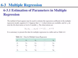
6-3 Multiple Regression. 6-3.1 Estimation of Parameters in Multiple Regression. 6-3 Multiple Regression. 6-3.1 Estimation of Parameters in Multiple Regression. The least squares function is given by. The least squares estimates must satisfy. 6-3 Multiple Regression.

6-3 Multiple Regression
E N D
Presentation Transcript
6-3 Multiple Regression 6-3.1 Estimation of Parameters in Multiple Regression
6-3 Multiple Regression 6-3.1 Estimation of Parameters in Multiple Regression • The least squares function is given by • The least squares estimates must satisfy
6-3 Multiple Regression 6-3.1 Estimation of Parameters in Multiple Regression • The least squares normal equations are • The solution to the normal equations are the least squares estimators of the regression coefficients.
6-3 Multiple Regression X’X in Multiple Regression
6-3 Multiple Regression 6-3.1 Estimation of Parameters in Multiple Regression
6-3 Multiple Regression Adjusted R2 We can adjust the R2 to take into account the number of regressors in the model: The ADJ RSQ does not always increase, like R2, as kincreases. ADJ RSQ is especially preferred to R2 if k/n is a large fraction (greater than 10%). If k/n is small, then both measures are almost identical. Always: ADJ RSQ R2 = 1 SSE/SS(TOTAL) ADJ RSQ = 1 – MSE/MS(TOTAL) where MS(TOTAL)=SS(TOTAL)/(n1) = sample variance of y.
6-3 Multiple Regression 6-3.2 Inferences in Multiple Regression Test for Significance of Regression
6-3 Multiple Regression 6-3.2 Inferences in Multiple Regression Inference on Individual Regression Coefficients • This is called a partial or marginal test
6-3 Multiple Regression 6-3.2 Inferences in Multiple Regression Confidence Intervals on the Mean Response and Prediction Intervals +
6-3 Multiple Regression Confidence Intervals on the Mean Response and Prediction Intervals The response at the point of interest is and the corresponding predicted value is + The prediction error is , and the standard deviation of this prediction error is
6-3 Multiple Regression 6-3.2 Inferences in Multiple Regression Confidence Intervals on the Mean Response and Prediction Intervals
6-3 Multiple Regression 6-3.3 Checking Model Adequacy Residual Analysis
6-3 Multiple Regression 6-3.3 Checking Model Adequacy Residual Analysis
6-3 Multiple Regression 6-3.3 Checking Model Adequacy Residual Analysis
6-3 Multiple Regression 6-3.3 Checking Model Adequacy Residual Analysis
6-3 Multiple Regression 6-3.3 Checking Model Adequacy Residual Analysis Because the ’s are always between zero and unity, a studentized residual is always larger than the corresponding standardized residual. Consequently, studentized residuals are a more sensitive diagnostic when looking for outliers.
6-3 Multiple Regression 6-3.3 Checking Model Adequacy Influential Observations • The disposition of points in the x-space is important in determining the properties of the model in R2, the regression coefficients, and the magnitude of the error mean squares. • A large value of Di implies that the ith points is influential. • A value of Di>1 would indicate that the point is influential.
6-3 Multiple Regression 6-3.3 Checking Model Adequacy
6-3 Multiple Regression Example 6-7 OPTIONS NOOVP NODATE NONUMBER LS=140; DATA ex67; INPUT strength length height @@; CARDS; 9.95 2 50 24.45 8 110 31.75 11 120 35 10 550 25.02 8 295 16.86 4 200 14.38 2 375 9.6 2 52 24.35 9 100 27.5 8 300 17.08 4 412 37 11 400 41.95 12 500 11.66 2 360 21.65 4 205 17.89 4 400 69 20 600 10.3 1 585 34.93 10 540 46.59 15 250 44.88 15 290 54.12 16 510 56.63 17 590 22.13 6 100 21.15 5 400 PROCSGSCATTER data=ex67; MATRIX STRENGTH LENGTH HEIGHT; TITLE 'Scatter Plot Matrix for Wire Bond Data'; PROCREG data=ex67; MODEL strength=length height/xpx r CLB CLM CLI; PLOT npp.*Residual.; /* Normal Probability Plot */ PLOT RESIDual.*Pred.; /* Residual Plot */ PLOT Residual.*length; PLOT Residual.*height; TITLE 'Multiple Regression'; RUN; QUIT;
6-3 Multiple Regression The REG Procedure Model: MODEL1 Model Crossproducts X'X X'Y Y'Y Variable Intercept length height strength Intercept 25 206 8294 725.82 length 206 2396 77177 8008.47 height 8294 77177 3531848 274816.71 strength 725.82 8008.47 274816.71 27178.5316 ----------------------------------------------------------------------------------------------------------------------------------------------------- Multiple Regression The REG Procedure Model: MODEL1 Dependent Variable: strength Number of Observations Read 25 Number of Observations Used 25 Analysis of Variance Sum of Mean Source DF Squares Square F Value Pr > F Model 2 5990.77122 2995.38561 572.17 <.0001 Error 22 115.17348 5.23516 Corrected Total 24 6105.94470 Root MSE 2.28805 R-Square 0.9811 Dependent Mean 29.03280 Adj R-Sq 0.9794 CoeffVar 7.88090 Parameter Estimates Parameter Standard Variable DF Estimate Error t Value Pr > |t| 95% Confidence Limits Intercept 1 2.26379 1.06007 2.14 0.0441 0.06535 4.46223 length 1 2.74427 0.09352 29.34 <.0001 2.55031 2.93823 height 1 0.01253 0.00280 4.48 0.0002 0.00672 0.01833
6-3 Multiple Regression Multiple Regression The REG Procedure Model: MODEL1 Dependent Variable: strength Output Statistics Dependent Predicted Std Error Std Error Student Cook's Obs Variable Value Mean Predict 95% CL Mean 95% CL Predict Residual ResidualResidual -2-1 0 1 2 D 1 9.9500 8.3787 0.9074 6.4968 10.2606 3.2740 13.4834 1.5713 2.100 0.748 | |* | 0.035 2 24.4500 25.5960 0.7645 24.0105 27.1815 20.5930 30.5990 -1.1460 2.157 -0.531 | *| | 0.012 3 31.7500 33.9541 0.8620 32.1665 35.7417 28.8834 39.0248 -2.2041 2.119 -1.040 | **| | 0.060 4 35.0000 36.5968 0.7303 35.0821 38.1114 31.6158 41.5778 -1.5968 2.168 -0.736 | *| | 0.021 5 25.0200 27.9137 0.4677 26.9437 28.8836 23.0704 32.7569 -2.8937 2.240 -1.292 | **| | 0.024 6 16.8600 15.7464 0.6261 14.4481 17.0448 10.8269 20.6660 1.1136 2.201 0.506 | |* | 0.007 7 14.3800 12.4503 0.7862 10.8198 14.0807 7.4328 17.4677 1.9297 2.149 0.898 | |* | 0.036 8 9.6000 8.4038 0.9039 6.5291 10.2784 3.3018 13.5058 1.1962 2.102 0.569 | |* | 0.020 9 24.3500 28.2150 0.8185 26.5175 29.9125 23.1754 33.2546 -3.8650 2.137 -1.809 | ***| | 0.160 10 27.5000 27.9763 0.4651 27.0118 28.9408 23.1341 32.8184 -0.4763 2.240 -0.213 | | | 0.001 11 17.0800 18.4023 0.6960 16.9588 19.8458 13.4425 23.3621 -1.3223 2.180 -0.607 | *| | 0.013 12 37.0000 37.4619 0.5246 36.3739 38.5498 32.5936 42.3301 -0.4619 2.227 -0.207 | | | 0.001 13 41.9500 41.4589 0.6553 40.0999 42.8179 36.5230 46.3948 0.4911 2.192 0.224 | | | 0.001 14 11.6600 12.2623 0.7689 10.6678 13.8568 7.2565 17.2682 -0.6023 2.155 -0.280 | | | 0.003 15 21.6500 15.8091 0.6213 14.5206 17.0976 10.8921 20.7260 5.8409 2.202 2.652 | |***** | 0.187 16 17.8900 18.2520 0.6785 16.8448 19.6592 13.3026 23.2014 -0.3620 2.185 -0.166 | | | 0.001 17 69.0000 64.6659 1.1652 62.2494 67.0824 59.3409 69.9909 4.3341 1.969 2.201 | |**** | 0.565 18 10.3000 12.3368 1.2383 9.7689 14.9048 6.9414 17.7323 -2.0368 1.924 -1.059 | **| | 0.155 19 34.9300 36.4715 0.7096 34.9999 37.9431 31.5034 41.4396 -1.5415 2.175 -0.709 | *| | 0.018 20 46.5900 46.5598 0.8780 44.7389 48.3807 41.4773 51.6423 0.0302 2.113 0.0143 | | | 0.000 21 44.8800 47.0609 0.8238 45.3524 48.7694 42.0176 52.1042 -2.1809 2.135 -1.022 | **| | 0.052 22 54.1200 52.5613 0.8432 50.8127 54.3099 47.5042 57.6183 1.5587 2.127 0.733 | |* | 0.028 23 56.6300 56.3078 0.9771 54.2814 58.3342 51.1481 61.4675 0.3222 2.069 0.156 | | | 0.002 24 22.1300 19.9822 0.7557 18.4149 21.5494 14.9850 24.9794 2.1478 2.160 0.995 | |* | 0.040 25 21.1500 20.9963 0.6176 19.7153 22.2772 16.0813 25.9112 0.1537 2.203 0.0698 | | | 0.000 Sum of Residuals 0 Sum of Squared Residuals 115.17348 Predicted Residual SS (PRESS) 156.16295
6-3 Multiple Regression 6-3.3 Checking Model Adequacy Multicollinearity Multicollinearity is a catch-all phase referring to problems caused by the independent variables being correlated with each other. This can cause a number of problems Individual F-tests can be non-significant for important variables. The sign of a can be flopped. Recall, the partial slopes measure the change in Y for a unit change in the holding the other X’s constant. If two X’s are highly correlated, this interpretation doesn’t do much good. The MSE can be inflated. Also the SE’s of the partial slopes are inflated. Removing one X from the model may make another more significant or less significant.
6-3 Multiple Regression 6-3.3 Checking Model Adequacy Variance Inflation Factor The Quantity called the variance inflation factor is denoted as VIF(Xj). The larger the value of VIF(Xj), the more the multicollinearity and the larger the standard error of the due to having Xj in the model. A common rule of thumb is that if VIF(Xj)>5 then multicollinearity is high. Also 10 has been proposed (see Kutner book referenced below) as a cut off value. Mallow’s CP Another measure of the amount of multicollinearity is Mallow’s CP. Assume we have a total of r variables. Suppose we fit a model with only p of the r variables. Let SSEP be the sums of squares error from the p variable model and MSE the mean square error from the model with all r variables. Then We want CP to be near p+1 for a good model.
6-3 Multiple Regression 6-3.3 Checking Model Adequacy Multicollinearity
6-3 Multiple Regression Example OPTIONS NOOVP NODATE NONUMBER LS=100; DATA appraise; INPUT price units age size parking area cond$ @@; CARDS; 90300 4 82 4635 0 4266 F 384000 20 13 17798 0 14391 G 157500 5 66 5913 0 6615 G 676200 26 64 7750 6 34144 E 165000 5 55 5150 0 6120 G 300000 10 65 12506 0 14552 G 108750 4 82 7160 0 3040G 276538 11 23 5120 0 7881 G 420000 20 18 11745 20 12600G 950000 62 71 21000 3 39448 G 560000 26 74 11221 0 30000G 268000 13 56 7818 13 8088 F 290000 9 76 4900 0 11315 E 173200 6 21 5424 6 4461 G 323650 11 24 11834 8 9000 G 162500 5 19 5246 5 3828 G 353500 20 62 11223 2 13680 F 134400 4 70 5834 0 4680 E 187000 8 19 9075 0 7392 G 93600 4 82 6864 0 3840 F 110000 4 50 4510 0 3092 G 573200 14 10 11192 0 23704 E 79300 4 82 7425 0 3876 F 272000 5 82 7500 0 9542 E PROCCORR DATA=APPRAISE; VAR PRICE UNITS AGE SIZE PARKING AREA; TITLE 'CORRELATIONS OF VARIABLES IN MODEL'; PROCREG DATA=APPRAISE; MODEL PRICE=UNITS AGE SIZE PARKING AREA/R VIF; PLOT (RESIDUAL. STUDENT.)*PRED.; TITLE 'ALL VARIABLES IN MODEL'; PROCREG DATA=APPRAISE; MODEL PRICE=UNITS AGE AREA/R INFLUENCE; PLOT (RESIDUAL. STUDENT.)*PRED.; TITLE 'REDUCED MODEL'; RUN; QUIT;
6-3 Multiple Regression CORRELATIONS OF VARIABLES IN MODEL CORR 프로시저 6 Variables: price units age size parking area 단순 통계량 변수 N 평균 표준편차 합 최소값 최대값 price 24 296193 214164 7108638 79300 950000 units 24 12.50000 12.73475 300.00000 4.00000 62.00000 age 24 52.75000 26.43655 1266 10.00000 82.00000 size 24 8702 4221 208843 4510 21000 parking 24 2.62500 5.01140 63.00000 0 20.00000 area 24 11648 10170 279555 3040 39448 피어슨 상관 계수, N = 24 H0: Rho=0 가정하에서 Prob > |r| price units age size parking area price 1.00000 0.92207 -0.11118 0.73582 0.21385 0.96784 <.0001 0.6050 <.0001 0.3157 <.0001 units 0.92207 1.00000 -0.00982 0.79583 0.21290 0.87622 <.0001 0.9637 <.0001 0.3179 <.0001 age -0.11118 -0.00982 1.00000 -0.18563 -0.36141 0.03090 0.6050 0.9637 0.3852 0.0827 0.8860 size 0.73582 0.79583 -0.18563 1.00000 0.15151 0.66741 <.0001 <.0001 0.3852 0.4797 0.0004 parking 0.21385 0.21290 -0.36141 0.15151 1.00000 0.07830 0.3157 0.3179 0.0827 0.4797 0.7161 area 0.96784 0.87622 0.03090 0.66741 0.07830 1.00000 <.0001 <.0001 0.8860 0.0004 0.7161
6-3 Multiple Regression ALL VARIABLES IN MODEL The REG Procedure Model: MODEL1 Dependent Variable: price Number of Observations Read 24 Number of Observations Used 24 Analysis of Variance Sum of Mean Source DF Squares Square F Value Pr > F Model 5 1.033962E12 2.067924E11 177.60 <.0001 Error 18 20959224743 1164401375 Corrected Total 23 1.054921E12 Root MSE 34123 R-Square 0.9801 Dependent Mean 296193 Adj R-Sq 0.9746 CoeffVar 11.52063 Parameter Estimates Parameter Standard Variance Variable DF Estimate Error t Value Pr > |t| Inflation Intercept 1 93629 29874 3.13 0.0057 0 units 1 4156.17223 1532.28739 2.71 0.0143 7.52119 age 1 -856.06670 306.65871 -2.79 0.0121 1.29821 size 1 0.88901 2.96966 0.30 0.7681 3.10362 parking 1 2675.62291 1626.23661 1.65 0.1173 1.31193 area 1 15.53982 1.50259 10.34 <.0001 4.61289
6-3 Multiple Regression REDUCED MODEL (NO SIZE AND PARKING) The REG Procedure Model: MODEL1 Dependent Variable: price Number of Observations Read 24 Number of Observations Used 24 Analysis of Variance Sum of Mean Source DF Squares Square F Value Pr > F Model 3 1.03081E12 3.436033E11 285.01 <.0001 Error 20 24111264632 1205563232 Corrected Total 23 1.054921E12 Root MSE 34721 R-Square 0.9771 Dependent Mean 296193 Adj R-Sq 0.9737 CoeffVar 11.72249 Parameter Estimates Parameter Standard Variable DF Estimate Error t Value Pr > |t| Intercept 1 114857 17919 6.41 <.0001 units 1 5012.58292 1183.19286 4.24 0.0004 age 1 -1054.84586 274.79652 -3.84 0.0010 area 1 14.96564 1.48218 10.10 <.0001
6-3 Multiple Regression ALL VARIABLES IN MODEL The REG Procedure Model: MODEL1 Dependent Variable: price Output Statistics Dependent Predicted Std Error Std Error Student Cook's Obs Variable Value Mean Predict Residual ResidualResidual -2-1 0 1 2 D 1 90300 110470 12281 -20170 31837 -0.634 | *| | 0.010 2 384000 405080 23185 -21080 25037 -0.842 | *| | 0.101 3 157500 165962 9178 -8462 32866 -0.257 | | | 0.001 4 676200 700437 25152 -24237 23061 -1.051 | **| | 0.219 5 165000 167009 10095 -2009 32596 -0.0616 | | | 0.000 6 300000 316800 17858 -16800 29077 -0.578 | *| | 0.021 7 108750 93663 13018 15087 31543 0.478 | | | 0.006 8 276538 246679 19376 29859 28088 1.063 | |** | 0.090 9 420000 421099 25938 -1099 22173 -0.0496 | | | 0.001 10 950000 930242 31527 19758 13057 1.513 | |*** | 2.225 11 560000 614511 17207 -54511 29467 -1.850 | ***| | 0.194 12 268000 267139 18075 860.6816 28943 0.0297 | | | 0.000 13 290000 246163 11851 43837 31999 1.370 | |** | 0.043 14 173200 190788 14200 -17588 31028 -0.567 | *| | 0.011 15 323650 290586 14788 33064 30752 1.075 | |** | 0.045 16 162500 175673 14612 -13173 30836 -0.427 | | | 0.007 17 353500 351590 10164 1910 32575 0.0586 | | | 0.000 18 134400 128242 9951 6158 32640 0.189 | | | 0.001 19 187000 233552 13949 -46552 31142 -1.495 | **| | 0.075 20 93600 105832 12433 -12232 31778 -0.385 | | | 0.004 21 110000 119509 12404 -9509 31789 -0.299 | | | 0.002 22 573200 521561 22525 51639 25632 2.015 | |**** | 0.522 23 79300 106890 12957 -27590 31567 -0.874 | *| | 0.021 24 272000 199161 13080 72839 31517 2.311 | |**** | 0.153 Sum of Residuals 0 Sum of Squared Residuals 20959224743 Predicted Residual SS (PRESS) 56380131094
6-3 Multiple Regression Consider the Full Model vs: 98.01% of the variability in the Y’s is explained by the relation to the X’s. The adjusted R2 is 0.9746 which is very close to the R2 value. This indicates no serious problems with the number of independent variables. Possible multicollinearity between units, area and size since they have large correlations. Age and parking have low correlations with price so may not be needed.
6-3 Multiple Regression We have some evidence of multicollinearity, thus we must consider dropping some of the variables. Let’s look at the individual tests of vs: , i=1, 2, These tests are summarized in the SAS output of PROC REG. Size is very non-significant (p-value=0.7681) and parking is also not significant (p-value=0.1173). There is evidence from the correlations that size is related to both units and area, so removing this variable might remove much of the multicollinearity. Parking just doesn’t seem to explain much variability in price. Let’s look at a 95% confidence interval for . ) 2675(2.101)*(1626.24) (741.1, 6092.4)
6-3 Multiple Regression A Test for the Significance of a Group of Regressors (Partial F-Test) Suppose that the full model has kregressors, and we are interested in testing whether the last k-r of them can be deleted from the model. This smaller model is called the reduced model. That is, the full model is and the reduced model has ==0, so the reduced model is Then, to test the hypotheses
6-3 Multiple Regression Testing The Full model is The Reduced model is From the SAS output we have No evidence to reject the null hypothesis.
6-3 Multiple Regression Interpreting the ’s For the apartment appraisal problem we have The ’s are = 114,857.4 =5,012.6 (units) (age)=14.96 (area) If one extra unit is added (all other factors held constant) the value of the complex will increase by $5,012.6. If the complex ages one more year it will lose $1,054.0 in value (all other factors held constant). If the area is increased by one square feet the value of the complex will increase by $14.96 (all other factors held constant). Notice the potential for multicollinearity. If one more unit is added, the number of square feet would also increase. Thus the interdependency of some of the variables makes the ’s harder to interpret.
6-3 Multiple Regression Notes on the Reduced Model The MSE has increased in the reduced model (MSE=34,721) vs. the full model(MSE=34,123), but the standard error of the individual ’s have all decreased. This is another indication that there was multicollinearity in the full model. We will be able to do more accurate influence in this reduced model. The R2and adjusted R2have been decreased by only a small amount. This justified dropping the two variables, also. All the individual ’s are significantly different from zero (all p-values small). This indicates that we probably cannot remove further variables without losing some information about the Y’s.
6-3 Multiple Regression Examining the Final Model Some final checks on the model are: Residual Studentized (standardized) residuals The studentized residuals should be between -2 and 2 around 95% of the time. If an excessive number of greater than 2 in absolute value or if any one studentized residual is much greater than 2 you should investigate closer. 3) Hat diagonals are the main diagonal element of the matrix We have already seen that is important. The diagonal elements as well as the eigen values of this matrix contain much information. Each diagonal corresponds to a particular observation. Look for values of the diagonal that are greater than 1.
6-3 Multiple Regression One More Diagnostic DFFITS This diagnostic investigates the influence of each observation on the value of the parameters. The parameters are first fit with all observations, call the parameter . Next the parameters are estimated using all but the jth observation. Call these estimated . The DFFITS for the ithparameter and jth observation is calculated as You look for values of DFFITS that are much larger than the other values. This indicates that the observation is too influential in determining the value of the parameters. A combined DFFITS can also be calculated which looks at all the parameters at once.
6-3 Multiple Regression REDUCED MODEL The REG Procedure Model: MODEL1 Dependent Variable: price Output Statistics Dependent Predicted Std Error Std Error Student Cook's Obs Variable Value Mean Predict Residual ResidualResidual -2-1 0 1 2 D 1 90300 112254 12030 -21954 32570 -0.674 | *| | 0.015 2 384000 416767 13928 -32767 31805 -1.030 | **| | 0.051 3 157500 169298 9015 -11798 33530 -0.352 | | | 0.002 4 676200 688661 21982 -12461 26877 -0.464 | | | 0.036 5 165000 173494 8304 -8494 33714 -0.252 | | | 0.001 6 300000 314198 10357 -14198 33141 -0.428 | | | 0.004 7 108750 93906 12575 14844 32364 0.459 | | | 0.008 8 276538 263679 11347 12859 32815 0.392 | | | 0.005 9 420000 384689 13763 35311 31877 1.108 | |** | 0.057 10 950000 941108 31332 8892 14961 0.594 | |* | 0.387 11 560000 616095 17479 -56095 30001 -1.870 | ***| | 0.297 12 268000 241992 9249 26008 33467 0.777 | |* | 0.012 13 290000 249139 10066 40861 33230 1.230 | |** | 0.035 14 173200 189543 12261 -16343 32484 -0.503 | *| | 0.009 15 323650 279370 10773 44280 33008 1.341 | |** | 0.048 16 162500 177167 12803 -14667 32275 -0.454 | | | 0.008 17 353500 354439 9992 -938.6096 33252 -0.0282 | | | 0.000 18 134400 131108 9953 3292 33264 0.0990 | | | 0.000 19 187000 245542 11977 -58542 32590 -1.796 | ***| | 0.109 20 93600 105878 12192 -12278 32510 -0.378 | | | 0.005 21 110000 128439 9416 -18439 33420 -0.552 | *| | 0.006 22 573200 529231 22052 43969 26819 1.639 | |*** | 0.454 23 79300 106417 12177 -27117 32516 -0.834 | *| | 0.024 24 272000 196225 12163 75775 32521 2.330 | |**** | 0.190

