Chapter 3 Multiple Linear Regression
Chapter 3 Multiple Linear Regression. Ray-Bing Chen Institute of Statistics National University of Kaohsiung. 3.1 Multiple Regression Models. Multiple regression model: involve more than one regressor variable.

Chapter 3 Multiple Linear Regression
E N D
Presentation Transcript
Chapter 3 Multiple Linear Regression Ray-Bing Chen Institute of Statistics National University of Kaohsiung
3.1 Multiple Regression Models • Multiple regression model: involve more than one regressor variable. • Example: The yield in pounds of conversion depends on temperature and the catalyst concentration.
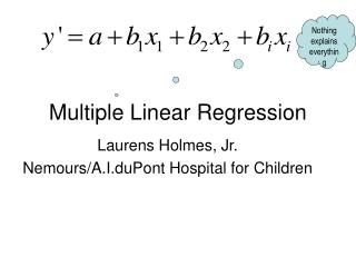
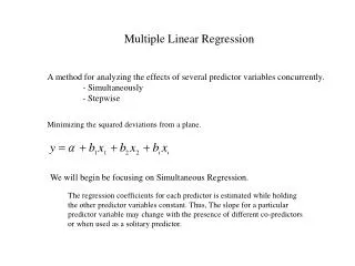
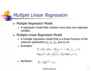
The response y may be related to k regressor or predictor variables: (multiple linear regression model) • The parameter j represents the expected change in the response y per unit change in xiwhen all of the remaining regressor variables xj are held constant.
Multiple linear regression models are often used as the empirical models or approximating functions. (True model is unknown) • The cubic model: • The model with interaction effects: • Any regression model that is linear in the parameters is a linear regression model, regardless of the shape of the surface that it generates.
3.2 Estimation of the Model Parameters 3.2.1 Least-squares Estimation of the Regression Coefficients • n observations (n > k) • Assume • The error term , E() = 0 and Var() = 2 • The errors are uncorrelated. • The regressor variables, x1,…, xk are fixed.
The sample regression model: • The least-squares function: • The normal equations:
The fitted model corresponding to the levels of the regressor variable, x: • The hat matrix, H, is an idempotent matrix and is a symmetric matrix. i.e. H2 = H and HT = H • H is an orthogonal projection matrix. • Residuals:
Example 3.1 The Delivery Time Data • y: the delivery time, • x1: the number of cases of product stocked, • x2: the distance walked by the route driver • Consider y = 0 + 1 x1 + 2 x2 +
3.2.2 A Geometrical Interpretation of Least Square • y = (y1,…,yn) is the vector of observations. • X contains p (p = k+1) column vectors (n ×1), i.e. X = (1,x1,…,xk) • The column space of X is called the estimation space. • Any point in the estimation space is X. • Minimize square distance S()=(y-X)’(y-X)
3.2.3 Properties of the Least Square Estimators • Unbiased estimator: • Covariance matrix: • Let C=(X’X)-1 • The LSE is the best linear unbiased estimator • LSE = MLE under normality assumption
3.2.4 Estimation of 2 • Residual sum of squares: • The degree of freedom: n – p • The unbiased estimator of 2: Residual mean squares
Example 3.2 The Delivery Time Data • Both estimates are in a sense correct, but they depend heavily on the choice of model. • The model with small variance would be better.
3.2.5 Inadequacy of Scatter Diagrams in Multiple Regression • For the simple linear regression, the scatter diagram is an important tool in analyzing the relationship between y and x. • However it may not be useful in multiple regression. • y = 8 – 5 x1 + 12 x2 • The y v.s. x1 plot do not exhibit any apparent relationship between y and x1 • The y v.s. x2 plot indicates the linear relationship with the slope 8.
In this case, constructing scatter diagrams of y v.s. xj (j = 1,2,…,k) can be misleading. • If there is only one (or a few) dominant regressor, or if the regressors operate nearly independently, the matrix scatterplots is most useful.
3.2.6 Maximum-Likelihood Estimation • The Model is y = X + • ~N(0, 2I) • The likelihood function and log-likelihood function: • The MLE of 2
3.3 Hypothesis Testing in Multiple Linear Regression • Questions: • What is the overall adequacy of the model? • Which specific regressors seem important? • Assume the errors are independent and follow a normal distribution with mean 0 and variance 2
3.3.1 Test for Significance of Regression • Determine if there is a linear relationship between y and xj, j = 1,2,…,k. • The hypotheses are H0: β1 = β2 =…= βk = 0 H1: βj 0 for at least one j • ANOVA • SST = SSR + SSRes • SSR/2 ~ 2k, SSRes/2 ~ 2n-k-1, and SSR and SSRes are independent
Under H1, F0 follows F distribution with k and n-k-1 and a noncentrality parameter of
R2 and Adjusted R2 • R2 always increase when a regressor is added to the model, regardless of the value of the contribution of that variable. • An adjusted R2: • The adjusted R2 will only increase on adding a variable to the model if the addition of the variable reduces the residual mean squares.
3.3.2 Tests on Individual Regression Coefficients • For the individual regression coefficient: • H0: βj = 0 v.s. H1: βj 0 • Let Cjj be the j-th diagonal element of (X’X)-1. The test statistic: • This is a partial or marginal test because any estimate of the regression coefficient depends on all of the other regression variables. • This test is a test of contribution of xj given the other regressors in the model
For the full model, the regression sum of square • Under the null hypothesis, the regression sum of squares for the reduce model • The degree of freedom is p-r for the reduce model. • The regression sum of square due to β2 given β1 • This is called the extra sum of squares due to β2 and the degree of freedom is p - (p - r) = r • The test statistic
If β2 0, F0 follows a noncentral F distribution with • Multicollinearity: this test actually has no power! • This test has maximal power when X1 and X2 are orthogonal to one another! • Partial F test: Given the regressors in X1, measure the contribution of the regressors in X2.
Consider y = β0 + β1 x1 + β2 x2 + β3 x3 + SSR(β1| β0 , β2, β3), SSR(β2| β0 , β1, β3) and SSR(β3| β0 , β2, β1) are signal-degree-of –freedom sums of squares. • SSR(βj| β0 ,…, βj-1, βj, … βk) : the contribution of xj as if it were the last variable added to the model. • This F test is equivalent to the t test. • SST = SSR(β1 ,β2, β3|β0) + SSRes • SSR(β1 ,β2 , β3|β0) = SSR(β1|β0) + SSR(β2|β1, β0) + SSR(β3 |β1, β2, β0)
3.3.3 Special Case of Orthogonal Columns in X • Model: y = Xβ + = X1β1+ X2β2 + • Orthogonal: X1’X2 = 0 • Since the normal equation (X’X)β= X’y,
3.3.4 Testing the General Linear Hypothesis • Let T be an m p matrix, and rank(T) = r • Full model: y = Xβ + • Reduced model: y = Z + , Z is an n (p-r) matrix and is a (p-r) 1 vector. Then • The difference: SSH = SSRes(RM) – SSRes(FM)with r degree of freedom. SSH is called the sum of squares due to the hypothesis H0: Tβ = 0
Another form: • H0: Tβ = c v.s. H1: Tβ c Then

