Multiple linear regression
Multiple linear regression. So far we have been dealing with a single predictor and a single response – simple linear regression When we have multiple predictors we talk about multiple linear regression Multiple linear regression is just as easy to perform as simple linear regression

Multiple linear regression
E N D
Presentation Transcript
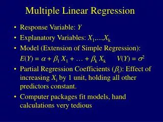
Multiple linear regression • So far we have been dealing with a single predictor and a single response – simple linear regression • When we have multiple predictors we talk about multiple linear regression • Multiple linear regression is just as easy to perform as simple linear regression • But there are a few more problems that can occur • And we have to think much more about the process of model selection • Model selection is possibly one of the hardest problems in statistics Statistical Data Analysis - Lecture20 - 07/05/03
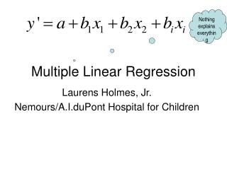
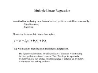
A probability model for multiple linear regression • Now instead of one predictor we have p. Our model becomes • Note our model still has an intercept, and, it makes the same assumptions about the distribution of the residuals • If we rewrite this in matrix form we write • This looks just the same as before, but in fact some of the definitions have changed slightly Statistical Data Analysis - Lecture20 - 07/05/03
Matrix form of regression model for multiple linear regression • Lety be a (n by 1) vector of responses, y= (y1,y2,…,yn)T • Letbe a (n by 1) vector of errors, = (1, 2,…, n)T • These are the same but now we let be a (p+1 by 1) vector of coefficients Xis called the design matrix and This form is convenient because the least squares solutions are found in exactly the same way as before Statistical Data Analysis - Lecture20 - 07/05/03
Changes to the Regression ANOVA and Regression Table • Our hypothesis for the ANOVA changes to H0: 1 = 2 =… = p=0 • Of course the alternative is now H1: i 0 for some i = 1,…,p • And a small P-value is evidence against the null hypothesis, i.e. evidence that the regression is significant • There is now a t-test associated with each regression coefficient, with small P-values implying that the specific predictors are important in predicting the response Statistical Data Analysis - Lecture20 - 07/05/03
Example • The data in this example were collected from 31 cherry trees in Allegheny National Forest, PA. • The measurements recorded were • Height in feet • Diameter in inches – we convert this to feet by dividing by 12 • Volume in cubic feet • The reason for this data collection was to estimate the volume (and therefore the total timber yield) of a tree given height and diameter Statistical Data Analysis - Lecture20 - 07/05/03
Model • If we let • v = Volume • d = Diameter • h = Height • then we could fit the following model to the data • Is this sensible? Statistical Data Analysis - Lecture20 - 07/05/03
Predictor Coef StDev T P Constant -57.988 8.638 -6.71 0.000 Diameter 56.498 3.171 17.82 0.000 Height 0.3393 0.1302 2.61 0.014 S = 3.882 R-Sq = 94.8% R-Sq(adj) = 94.4% Analysis of Variance Source DF SS MS F P Regression 2 7684.2 3842.1 254.97 0.000 Residual Error 28 421.9 15.1 Total 30 8106.1 • Looking at just the regression output, we can see • The P-value in the ANOVA table is small => the regression is significant • Each of the P-values for the terms in the regression table is significant => both height and diameter are important in predicting volume • The adj-R2 is 94.4% - pretty good • Is this a good model? Statistical Data Analysis - Lecture20 - 07/05/03
There doesn’t appear to be anything wrong with the norplot of the residuals • The there is a little wobble but nothing significant • There don’t appear to be any extreme residuals • The pred-res plot tells us something is definitely out of whack • The “Nike Swoosh” shape tells us • that our variance assumption does not hold • There is some non-linear trend left in the residuals Statistical Data Analysis - Lecture20 - 07/05/03
A better model? • So what’s wrong with our model? • It doesn’t take into account what we know about trees, and the relationship between height, diameter and volume • It seems reasonable to assume that the bulk of the volume in a tree comes from its trunk • And the trunk is approximately cylindrical so • Can we use this to make a better model • YES Statistical Data Analysis - Lecture20 - 07/05/03
Height Diameter • We know that the area of a circle is r2 where r is the radius of the circle and the radius is half the diameter, i.e. r = d/2 • If the cylinder has height h, then the volume of the cylinder is the area of the circle times the height, i.e. • This is clearly a non-linear relationship • But it does have a simple multiplicative structure • If we take logs, then the relationship will become linear Statistical Data Analysis - Lecture20 - 07/05/03
Logarithms can help • By taking logarithms of each side we might get a sensible model, i.e. • When we propose our regression model, we now have some idea as to what we expect the coefficients to be • That is, if our cylinder model is true, then we expect 0 to be about –0.242, 1 2, and 2 1 Statistical Data Analysis - Lecture20 - 07/05/03
log(vol) = - 1.70 + 1.98 log(diam) + 1.12 log(height) Predictor Coef StDev T P Constant -1.7049 0.8819 -1.93 0.063 log(diam 1.98265 0.07501 26.43 0.000 log(heig 1.1171 0.2044 5.46 0.000 S = 0.08139 R-Sq = 97.8% R-Sq(adj) = 97.6% Analysis of Variance Source DF SS MS F P Regression 2 8.1232 4.0616 613.19 0.000 Residual Error 28 0.1855 0.0066 Total 30 8.3087 • From the regression table things look pretty good • The regression is significant • The adj-R2 is even higher than before • And the coefficients are almost what we expected them to be • The only surprise is that the constant is –1.70 << -0.242 Statistical Data Analysis - Lecture20 - 07/05/03
We might be a bit concerned about the three points that seem to be a little too far away in the norplot, but the magnitude of the residuals is a good indication that removing these points will have little effect on model fit. • The pred-res plot shows none of the banding we saw before – everything looks okay Statistical Data Analysis - Lecture20 - 07/05/03
The leverage plot looks pretty good as well • There are no observations that have a hat matrix diagonal of greater than 3(2+1)/31 = 0.290 and only 2 greater than 2(2+1)/31 = 0 Statistical Data Analysis - Lecture20 - 07/05/03
The fitted model • We’ve fitted a model, and checked that it is okay • But our “client” wants a to use this model to predict the timber volume of a specific cherry tree – given its height and diameter • Our model is in terms of logarithms, and, our client didn’t ask about the logarithm of the volume. • Therefore we need to re-state the model in a useable form • We could write • However, it is probably might be more use for the client to have a model that is rounded • Unfortunately this model significantly underestimates volume Statistical Data Analysis - Lecture20 - 07/05/03
An alternative • We didn’t need to take logarithms • If we were sure that the model was of the form • Then we could have constructed a new variable and fit the model • This is a “no intercept” model • These models are sometimes frowned upon However we do have justification for this type of model here, because it is reasonable to expect a tree with zero height or zero diameter to have zero volume Statistical Data Analysis - Lecture20 - 07/05/03
Some differences • There is a difference between this model and our previous model that may not be immediately obvious • In the previous model we unconsciously assumed that the errors were multiplicative, i.e. • So in our logarithm model we were saying the log of the errors is normal • In our second model we have additive errors • This type of error structure can cause us problems and you should be aware it • However, it doesn’t cause too much problem here Statistical Data Analysis - Lecture20 - 07/05/03
Model fit • Minitab doesn’t give R2 for models with no intercept, but it can be easily calculated using • Doing this gives R2 = 0.995, so this model certainly explains a large proportion of the variation (99.5%) • How well does it fit? • Let’s look at the usual measures Statistical Data Analysis - Lecture20 - 07/05/03
Predictor Coef StDev T P d2h 0.303567 0.003920 77.44 0.000 S = 2.455 Analysis of Variance Source DF SS MS F P Regression 1 36144 36144 5996.41 0.000 Residual Error 30 181 6 Total 31 36325 Statistical Data Analysis - Lecture20 - 07/05/03
Which model is better? • Welcome to the world of model selection. • It depends on your criteria • A model of the form 0.304d2h is probably easier to use than a model of the form 0.183d1.98h1.12 • And it has intuitive appeal in that it is very close the formula for a cone, • However, both models explain about the same percentage of variation and have similar residual standard deviations (2.451 vs. 2.455) Statistical Data Analysis - Lecture20 - 07/05/03

