Chapter 5 Multiple Linear Regression
Chapter 5 Multiple Linear Regression. Introduction. Fit a linear relationship between a quantitative dependent variable and a set of predictors. Assume the following relationship holds Review Simple Regression Example. Explanatory V.S. Predictive Modeling.

Chapter 5 Multiple Linear Regression
E N D
Presentation Transcript
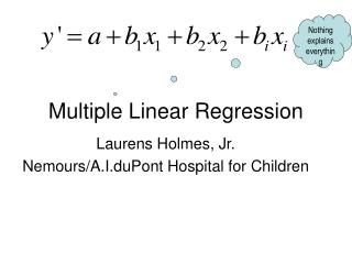
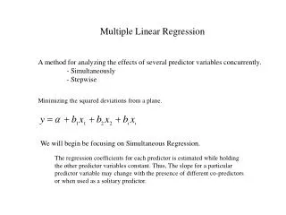
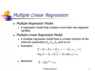
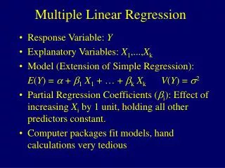
Introduction • Fit a linear relationship between a quantitative dependent variable and a set of predictors. • Assume the following relationship holds • Review Simple Regression Example
Explanatory V.S. Predictive Modeling • Both explanatory modeling and predictive modeling involve using a dataset to • Fit a model (i.e. to estimate coefficients), • checking model validity, • assessing its performance, and • comparing to other models.
Explanatory V.S. Predictive Modeling • There are several major differences between the two: • A good explanatory model is one that fits the data closely, whereas a good predictive model is one that accurately predicts new cases. • In explanatory models (classical statistical world, scarce data) the entire dataset is used for estimating the best-fit model, in order to maximize the amount of information that we have about the hypothesized relationship in the population. • When the goal is to predict outcomes of new cases (data mining, plentiful data), the data are typically split into training set and validation set. • The training set is used to estimate the model, • The holdout set is used to assess this model's performance on new, unobserved data.
Explanatory V.S. Predictive Modeling • Performance measures • explanatory models measure how close the data fit the model (how well the model approximates the data), • predictive models performance is measured by predictive accuracy (how well the model predicts new cases).
Explanatory V.S. Predictive Modeling • Know the goal of the analysis before beginning the modelling process. • A good predictive model can have a looser fit to the data it is based on, • A good explanatory model can have low prediction accuracy. • In data mining we focus on predictive models • Estimating the Regression Equation and Prediction • Example: Predicting the Price of Used Toyota Corolla Automobiles
Variable Selection in Linear Regression • Why Reduce the Number of Predictors • It may be expensive or not feasible to collect the full complement of predictors for future predictions. • We may be able to measure fewer predictors more accurately (e.g., in surveys). • The more predictors, the higher chance of missing values in the data. If we delete or impute cases with missing values, then multiple predictors will lead to a higher rate of case deletion or imputation. • Parsimony is an important property of good models. We obtain more insight into the influence of predictors in models with few parameters. • Estimates of regression coefficients are likely to be unstable due to multicollinearity in models with many variables. (Multicollinearity is the presence of two or more predictors sharing the same linear relationship with the outcome variable.) Regression coefficients are more stable for parsimonious models. One very rough rule of thumb is to have a number of cases n larger than 5(p + 2), where p is the number of predictors. • It can be shown that using predictors that are uncorrelated with the dependent variable in creases the variance of predictions. • It can be shown that dropping predictors that are actually correlated with the dependent variable can increase the average error (bias) of predictions.
Variable Selection in Linear Regression • How to Reduce the Number of Predictors • Exhaustive Search Controlled by • Adjusted R2 • Uses a penalty on the number of predictors • Equivalent to choosing subset that minimizes the variance in the predictions. • Mallow’s Cp • assumes that the full model (with all predictors) is unbiased although it may have predictors that, if dropped, would reduce prediction variability. • good models are those that have values of Cp near p + 1 and that have small p (i.e. are of small size) • See text for definition of Cp
Reduce Predictors Partial Iterative Search • Three Techniques: • “forward selection" • we start with no predictors, and then add predictors one by one. Each added predictor is the one (among all predictors) that has the largest contribution to the R2 on top of the predictors that are already in it. • The algorithm stops when the contribution of additional predictors is not statistically significant. • The main disadvantage of this method is that the algorithm will miss pairs or groups of predictors that perform very well together, but perform poorly as single predictors. • This is similar to interviewing job candidates for a team project one by one, thereby missing groups of candidates who perform superiorly together, but poorly on their own. • “backward elimination" • start with all predictors, and then at each step eliminate the least useful predictor (according to statistical significance). • algorithm stops when all the remaining predictors have significant contributions. • The weakness of this algorithm is that computing the initial model with all predictors can be time-consuming and unstable. • “stepwise” • like forward selection except that at each step we consider dropping predictors that are not statistically significant as in backward elimination.
Problems • Problem 5.1 Predicting Boston Housing Prices

