V. Regression Diagnostics
V. Regression Diagnostics. Regression analysis assumes a random sample of independent observations on the same individuals (i.e. units). What are its other basic assumptions? They all concern the residuals ( e ):.

V. Regression Diagnostics
E N D
Presentation Transcript
Regression analysis assumes a random sample of independent observations on the same individuals (i.e. units). • What are its other basic assumptions? They all concern the residuals (e):
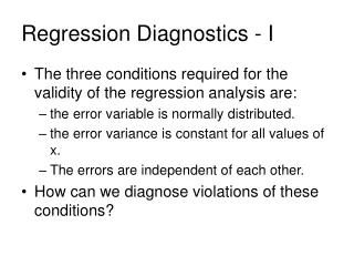
(1) The mean of the probability distribution of e over all possible samples is 0: i.e. the mean of e does not vary with the levels of x. (2) The variance of the probability distribution of e is constant for all levels of x: i.e. the variance of the residuals does not vary with the levels of x.
(3) The errors associated with any two different y observations are 0: i.e. the errors are uncorrelated—the errors associated with one value of y have no effect on the errors associated with other y values. (4) The probability distribution of e is normal.
The assumptions are commonly summarized as I.I.D.: independent & identically distributed residuals. • To the degree that these assumptions are confirmed, then the relationship between the outcome variable & independent variables is adequately linear.
What are the implications of these assumptions? • Assumption 1: ensures that the regression coefficients are unbiased. • Assumptions 2 & 3: ensure that the standard errors are unbiased & are the lowest possible, making p-values & significance tests trustworthy. • Assumption 4: ensures the validity of confidence intervals & p-values.
Assumption 4 is by far the least important: even if the distribution of a regession model’s residuals depart from approximate normality, the central limit theorem makes us generally confident that confidence intervals & p-values will be trustworthy approximations if the sample is at least 100-200. • Problems with assumption 4, however, may be indicative of problems with the other, crucial assumptions: when might these be violated to the degree that the findings are highly biased & unreliable?
Serious violations of assumption 1 result from anything that causes serious bias of the coefficients: examples? • Violations of assumption 2 occur, e.g., when variance of income increases as the value of income increases, or when variance of body weight increases as body weight itself increases: this pattern is commonplace.
Violations of assumption 3 occur as a result of clustered observations or time-series observations: variance is not independent from one observation to another but rather is correlated. • E.g., in a cluster sample of individuals from neighborhoods, schools, or households, the individuals within any such unit tend to be significantly more homogeneous than are individuals in the wider sample. Ditto for panel or time-series observations.
In the real world, the linear model is usually no better than an approximation, & violations to one extent or another are the norm. • What matters is if the violations surpass some critical threshold. • Regression diagnostics: procedures to detect violations of the linear model’s assumptions; gauge the severity of the violations; & take appropriate remedial action.
Keep in mind:statistical vs. practical significance in evaluating the findings of diagnostic tests. • See King et al. for applications of the logic of regression diagnostics to qualitative social science research as well.
Keep in mind that the linear model does not assume that the distribution of a variable’s observations is normal. • Its assumptions, rather, involve the residuals (which are the sample estimates of the population e). • While it’s important to inspect univariate & bivariate distributions, & to be careful about extreme outliers, recall that multiple regression expresses the joint, multivariate associations of x’s with y.
Let’s turn our attention to regression diagnostics. • For the sake of presenting the material, we’ll examine & respond to the diagnostic tests step by step. • In ‘real life,’ though, we should go through the entire set of diagnostic tests first & then use them fluidly & interactively to address the problems.
Model Specification • Does a regression model properly account for the relationship between the outcome & explanatory variables? • See Wooldridge, Introductory Econometrics, pages 289-94; Allison, Multiple Regression, pages 49-52, 123-25; Stata Reference G-M, pages 274-79; N-R, 363-65.
If a model is functionally misspecified, its slope coefficients may be seriously biased, either too low or too high. • We could then either under or overestimate the y/x relationship; & conclude incorrectly that a coefficient is insignificant or significant.
If this is a problem, perhaps the outcome variable needs to be redefined to properly account for the y/x relationships (e.g., from ‘miles per gallon’ to ‘gallons per mile’). • Or perhaps, e.g., ‘wage’ needs to be transformed to ‘log(wage)’. • And/or maybe not OLS but another kind of regression—e.g., quantile regression— should be used.
Let’s begin by exploring the variables we’ll use. . use WAGE1, clear . hist wage, norm . gr box wage, marker(1, mlab(id)) . su wage, d . ladder wage • Note that ‘ladder wage’ doesn’t suggest a transformation, but log wage is common for right skewness.
. gen lwage=ln(wage) • . su wage lwage • . hist lwage, norm • . gr box lwage, marker(1, mlab(id)) • While a log transformation makes wage’s distribution much more normal, it leaves an extreme low-value outlier, id=24. • Let’s inspect its profile:
. list id wage lwage educ exp tenure female nonwhite if id==24 • It’s a white female with 12 years of education, but earning a very low wage. • We don’t know if its wage is an error, we’ll keep an eye on id=24 for possible problems. • Let’s exam the independent variables: .
. hist educ . gr box educ, marker(1, mlab(id)) . su educ, d . sparl lwage educ . sparl lwage educ, quad . twoway qfitci lwage educ . gen educ2=educ^2 . su educ educ2
. hist exper, norm . gr box exper, marker(1, mlab(id)) . su exper, d . exper, ladder . sparl lwage exper . sparl lwage exper, quad . twoway qfitci lwage exper . gen exper2=exper^2 . su exper exper2
. hist tenure, norm • . gr box tenure, marker(1, mlab(id)) • . su tenure, d • . su tenure if tenure>=25 & tenure<. • Note that there are only 18 cases of tenure>=25, & increasingly fewer cases with greater tenure. • . ladder tenure • . sparl lwage tenure
. sparl lwage tenure, quad • Note that there are cases of tenure=0, which must be accommodated in a log transformation. . gen ltenure=ln(tenure + 1) . su tenure ltenure . sparl lwage tenure . sparl lwage tenure, quad . sparl lwage ltenure [i.e. transformed]
. twoway qfitcit lwage tenure • . twoway qfitcit lwage ltenure • What other options could be explored for educ, exper, & tenure? • The data do not include age, which could be an important factor, including as a control. . tab female, su(lwage) . ttest lwage, by(female)
. tab nonwhite, su(lwage) • . ttest lwage, by(nonwhite) • Although nonwhite tests insignificant, it might become significant in the model. • Let’s first test the model omitting the transformed version of the variables: . reg wage educ exper tenure female nonwhite
A form of model misspecification is omitted variables, which also causes biased slope coefficients (see Allison, Multiple Regression, pages 49-52). • Leaving key explanatory variables out means that we have not adequately controlled for important x effects on y. • Thus we may incorrectly detect or fail to detect y/x relationships.
In STATA we use ‘estat ovtest’ (also known as regression specification test, RESET) to indicate whether there are important omitted variables or not. • ‘estat ovtest’ adds polynomials to the model’s fitted values: we want it to test insignificant so that we fail to reject the null hypothesis that there are no important omitted variables. • We want to fail to reject the null hypothesis that the model has no omitted variables.
. reg wage educ exper tenure female nonwhite . estat ovtest • Ramsey RESET test using powers of the fitted values of wage • Ho: model has no omitted variables • F(3, 517) = 9.37 • Prob > F = 0.0000 • The model fails. Let’s add the transformed variables.
. reg lwage educ educ2 exper exper2 ltenure female nonwhite • . estat ovtest • . estat ovtest • Ramsey RESET test using powers of the fitted values of lwage • Ho: model has no omitted variables • F(3, 515) = 2.11 • Prob > F = 0.0984 • The model passes. Perhaps it would do better if age were available, and with other variables & other forms of these predictors.
estat ovtest is a decisive hurdle to clear. • Even so, passing any diagnostic test by no means guarantees that we’ve specified the best possible model, statistically or substantively. • It could be, again, that other models would be better in terms of statistical fit and/or substance.
Another way to test the model’s functional specification via ‘linktest’: it tests whether y is properly specified or not. • linktest’s ‘hatsq’ must test insignificant: we want to fail to reject the null hypothesis that y is specifed correctly.
. linktest --------------------------------------------------------------------------------------------------- lwage | Coef. Std. Err. t P>|t| [95% Conf. Interval] -------------+------------------------------------------------------------------------------------- _hat | .3212452 .3478094 0.92 0.356 -.36203 1.00452 _hatsq | .2029893 .1030452 1.97 0.049 .0005559 .4054228 _cons | .5407215 .2855868 1.89 0.059 -.0203167 1.10176 ----------------------------------------------------------------------------------------------------- • The model fails. Let’s try another model that uses categorized predictors.
. xi:reg lwage hs scol ccol exper exper2 i.tencat female nonwhite • . estat ovtest=.12 • . linktest=.15 • We’ll stick with this model—unless other diagnostics indicate problems. Again, too bad the data don’t include age.
Passing ovtest, linktest, or other diagnostic indicatorsdoes not mean that we’ve necessarily specified the best possible model—either statistically or substantively. • It merely means that the model has passed some minimal statistical threshold of data fitting.
At this stage it’s helpful to plot the model’s residual versus fitted values to obtain a graphic perspective on the model’s fit & problems.
. rvfplot, yline(0) ml(id) • Problems of heteroscedasticity?
So, even though the model passed linktest & estat ovtest, at least one basic problems remains to be overcome. • Let’s examine other assumptions.
The model specification tests have to do with biased slope coefficients, & thus with Assumption 1. • Next, though, let’s examine a potential model problem—multicollinearity—which in fact does not violate any of the regression assumptions.
Multicollinearity • Multicollinearity: high correlations between the explanatory variables. • Multicollinearity does not violate any linear model assumptions: if our objective were merely to predict values of y, there would be no need to worry about it. • But, like small sample or subsample size, it does inflate standard errors.
It thereby makes it tough to find out which of the explanatory variables has a signficant effect. • For confidence intervals, p-values, & hypothesis tests, then, it does cause problems.
Signs of multicollinearity: • High bivariate correlations (say, .80+) between the explanatory variables: but, because multiple regression expresses joint linear effects, such correlations (or their absence) aren’t reliable indicators. • Global F-test is significant, but none of the individual t-tests is significant. • Very large standard errors.
(4) Sign of coefficients may be opposite of hypothesized direction (but could be Simpson’s paradox, etc.) (5) Adding/deleting explanatory variables causes large changes in coefficients, particularly switches between positive & negative. The following indicators are more reliable because they better gauge the array of joint effects within a model:
(6) Post-model estimation (STATA command ‘vif’) - ‘VIF’>10: measures inflation in variance due to multicollinearity. • Square root of VIF: shows the amount of increase in an explanatory variable’s standard error due to multicollinearity. • (7) Post-model estimation (STATA command ‘vif’)- ‘Tolerance’<.10: reciprocal of VIF; measures extent of variance that is independent of other explanatory variables. • (8) Pre-model estimation (downloadable STATA command ‘collin’) – ‘Condition Number’>15 or especially >30. • .
. vif • Variable | VIF 1/VIF • -------------+----------------------------- • exper | 15.62 0.064013 • exper2 | 14.65 0.068269 • hsc | 1.88 0.532923 • _Itencat_3 | 1.83 0.545275 • ccol | 1.70 0.589431 • scol | 1.69 0.591201 • _Itencat_2 | 1.50 0.666210 • _Itencat_1 | 1.38 0.726064 • female | 1.07 0.934088 • nonwhite | 1.03 0.971242 • -------------+---------------------------- • Mean VIF | 4.23 • The seemingly troublesome scores for exper exper2 are an artifact of the quadratic form & pose no problem. The results look fine.
What would we do if there were a problem of multicollinearity?
Correct any inappropriate use of explanatory dummy variables or computed quantitative variables. • ‘Center’ the offending explanatory variables (see Mendenhall/Sincich), perhaps using STATA’s ‘center’ command. • Eliminate variables—but this might cause specification errors (see, e.g., ovtest). • Collect additional data—if you have a big bank account & plenty of time! • Group relevant variables into sets of variables (e.g., an index): how might we do this?
Learn how to do ‘principal components analysis’ or ‘principal factor analysis’ (see Hamilton). • Or do ‘ridge regression’ (see Mendenhall/ Sincich).
Let’s skip to Assumption 4: that the residuals are normally distributed. • While this is by far the least important assumption, examining the residuals at this stage—as we began to do with rvfplot—can tip us off to other problems.
Normal Distribution of Residuals • This is necessary for confidence intervals & p-values to be accurate. • But this is the least worrisome problem in general: if the sample is as large as 100-200, the central limit theorem says that confidence intervals & p-values will be good approximations of a normal distribution.
The most basic way to assess the normality of residuals is simply to plot the residuals via histogram, box or dotplot, kdensity, or normal quantile plot. • We’ll use studentized(a version of standardized)residuals because we can asses their distribution relative to the normal distribution: . predict rstu if e(sample), rstu . su rstu, d Note: to obtain unstandardized residuals— predict e if e(sample), resid