Multiple Regression Assumptions & Diagnostics

1. Multiple Regression Assumptions & Diagnostics

2. Regression: Outliers • Note: Even if regression assumptions are met, slope estimates can have problems • Example: Outliers -- cases with extreme values that differ greatly from the rest of your sample • More formally: “influential cases” • Outliers can result from: • Errors in coding or data entry • Highly unusual cases • Or, sometimes they reflect important “real” variation • Even a few outliers can dramatically change estimates of the slope, especially if N is small.

3. Regression: Outliers Extreme case that pulls regression line up 4 2 -2 -4 -4 -2 0 2 4 Regression line with extreme case removed from sample • Outlier Example:

4. Regression: Outliers • Strategy for identifying outliers: • 1. Look at scatterplots or regression partial plots for extreme values • Easiest. A minimum for final projects • 2. Ask SPSS to compute outlier diagnostic statistics • Examples: “Leverage”, Cook’s D, DFBETA, residuals, standardized residuals.

5. Regression: Outliers • SPSS Outlier strategy: Go to Regression – Save • Choose “influence” and “distance” statistics such as Cook’s Distance, DFFIT, standardized residual • Result: SPSS will create new variables with values of Cook’s D, DFFIT for each case • High values signal potential outliers • Note: This is less useful if you have a VERY large dataset, because you have to look at each case value.

7. Scatterplots Y axis 30 20 10 0 X axis 0 1 2 3 4 • Example: Study time and student achievement. • X variable: Average # hours spent studying per day • Y variable: Score on reading test

8. Outliers • Results with outlier:

9. Outlier Diagnostics • Residuals: The numerical value of the error • Error = distance that points falls from the line • Cases with unusually large error may be outliers • Note: residuals have many other uses! • Standardized residuals • Z-score of residuals… converts to a neutral unit • Often, standardized residuals larger than 3 are considered worthy of scrutiny • But, it isn’t the best outlier diagnostic.

10. Outlier Diagnostics • Cook’s D: Identifies cases that are strongly influencing the regression line • SPSS calculates a value for each case • Go to “Save” menu, click on Cook’s D • How large of a Cook’s D is a problem? • Rule of thumb: Values greater than: 4 / (n – k – 1) • Example: N=7, K = 1: Cut-off = 4/5 = .80 • Cases with higher values should be examined.

11. Outlier Diagnostics • Example: Outlier/Influential Case Statistics

12. Outliers • Results with outlier removed:

13. Regression: Outliers • Question: What should you do if you find outliers? Drop outlier cases from the analysis? Or leave them in? • Obviously, you should drop cases that are incorrectly coded or erroneous • But, generally speaking, you should be cautious about throwing out cases • If you throw out enough cases, you can produce any result that you want! So, be judicious when destroying data.

14. Regression: Outliers • Circumstances where it can be good to drop outlier cases: • 1. Coding errors • 2. Single extreme outliers that radically change results • Your results should reflect the dataset, not one case! • 3. If there is a theoretical reason to drop cases • Example: In analysis of economic activity, communist countries may be outliers • If the study is about “capitalism”, they should be dropped.

15. Regression: Outliers • Circumstances when it is good to keep outliers • 1. If they form meaningful cluster • Often suggests an important subgroup in your data • Example: Asian-Americans in a dataset on education • In such a case, consider adding a dummy variable for them • Unless, of course, research design is not interested in that sub-group… then drop them! • 2. If there are many • Maybe they reflect a “real” pattern in your data.

16. Regression: Outliers • When in doubt: Present results both with and without outliers • Or present one set of results, but mention how results differ depending on how outliers were handled • For final projects: Check for outliers! • At least with scatterplots • In the text: Mention if there were outliers, how you handled them, and the effect it had on results.

17. Multicollinearity • Another common regression problem: Multicollinearity • Definition: collinear = highly correlated • Multicollinearity = inclusion of highly correlated independent variables in a single regression model • Recall: High correlation of X variables causes problems for estimation of slopes (b’s) • Recall: variable denominators approach zero, coefficients may wrong/too large.

18. Multicollinearity • Multicollinearity symptoms: • Unusually large standard errors and betas • Compared to if both collinear variables aren’t included • Betas often exceed 1.0 • Two variables have the same large effect when included separately… but… • When put together the effects of both variables shrink • Or, one remains positive and the other flips sign • Note: Not all “sign flips” are due to multicollinearity!

19. Multicollinearity • What does multicollinearity do to models? • Note: It does not violate regression assumptions • But, it can mess things up anyway • 1. Multicollinearity can inflate standard error estimates • Large standard errors = small t-values = no rejected null hypotheses • Note: Only collinear variables are effected. The rest of the model results are OK.

20. Multicollinearity • What does multicollinearity do? • 2. It leads to instability of coefficient estimates • Variable coefficients may fluctuate wildly when a collinear variable is added • These fluctuations may not be “real”, but may just reflect amplification of “noise” and “error” • One variable may only be slightly better at predicting Y… but SPSS will give it a MUCH higher coefficient • Note: These only affect variables that are highly correlated. The rest of the model is OK.

21. Multicollinearity • Diagnosing multicollinearity: • 1. Look at correlations of all independent vars • Correlation of .7 is a concern, .8> is often a problem • But, sometimes problems aren’t always bivariate… and don’t show up in bivariate correlations • Ex: If you forget to omit a dummy variable • 2. Watch out for the “symptoms” • 3. Compute diagnostic statistics • Tolerances, VIF (Variance Inflation Factor).

22. Multicollinearity • Multicollinearity diagnostic statistics: • “Tolerance”: Easily computed in SPSS • Low values indicate possible multicollinearity • Start to pay attention at .4; Below .2 is very likely to be a problem • Tolerance is computed for each independent variable by regressing it on other independent variables.

23. Multicollinearity • If you have 3 independent variables: X1, X2, X3… • Tolerance is based on doing a regression: X1 is dependent; X2 and X3 are independent. • Tolerance for X1 is simply 1 minus regression R-square. • If a variable (X1) is highly correlated with all the others (X2, X3) then they will do a good job of predicting it in a regression • Result: Regression r-square will be high… 1 minus r-square will be low… indicating a problem.

24. Multicollinearity • Variance Inflation Factor (VIF) is the reciprocal of tolerance: 1/tolerance • High VIF indicates multicollinearity • Gives an indication of how much the Standard Error of a variable grows due to presence of other variables.

25. Multicollinearity • Solutions to multcollinearity • It can be difficult if a fully specified model requires several collinear variables • 1. Drop unnecessary variables • 2. If two collinear variables are really measuring the same thing, drop one or make an index • Example: Attitudes toward recycling; attitude toward pollution. Perhaps they reflect “environmental views” • 3. Advanced techniques: e.g., Ridge regression • Uses a more efficient estimator (but not BLUE – may introduce bias).

26. What is Model Specification? • Model Specification is two sets of choices: • The set of variables that we include in a model • The functional form of the relationships we specify • These are central theoretical choices • Can’t get the right answer if we ask the wrong question

27. What is the “Right” Model? • In truth, all our models are misspecified to some extent. • Our theories are always a simplification of reality, and all our measures are imperfect • Our task is to seek models that are reasonably well specified – keeps our errors relatively modest

28. Omitting Variables and Model Specification • These criteria give us our conceptual standards for determining when a variable must be included • A model must be included in a regression equation IF: • The variable is correlated with other X’s AND • The variable is also a cause of Y

29. The Meaning of b in Multiple Regression • Each element of the vector b is a slope coefficient for one of the X’s • Same as in bivariate context except that b1 is the expected change in Y for a 1 unit increase in X1, while holding X2…Xn constant • Thus b1 represents the direct effect of X1 on Y, controlling for X2…Xn

30. Imagine a true model where X1has a small effect on Y and is correlated with X2 that has a large effect on Y. Specifiying both variables can distinguish these effects Illustrating Omitted Variable Bias X1 Y X2

31. But when we run simple model excluding X2, we attribute all causal influence to X1 Coefficient is too big and variance of coefficient is too small Illustrating Omitted Variable Bias X1 Y

32. Omitted Variable Bias: Causes • This problem is explicitly theoretical rather than “statistical.” • No statistical test can reveal a specification error or omitted variable bias • Scholars can form hypotheses about other X’s that may be a source of omitted variable bias

33. Including Irrelevant Variables • In this case: • If b2=0, our estimate of b1 is not affected • If X1’X2=0, our estimate of b1 is not affected • But including X2 if it is not relevant does unnecessarily inflate the σb2

34. Including Irrelevant Variables: Consequences • σb2 increases for two reasons: • Addition of parameter for X2 reduces the degrees of freedom • Part of estimator for σu2 • If b2=0 but X1’X2 is not, then including X2 unnecessarily reduces independent variation of X1 • Thus parsimony remains a virtue

35. Rules for Model Specification • Model specification is fundamentally a theoretical exercise. We build models to reflect our theories • Theorizing process cannot be replaced with statistical tests • Avoid mechanistic rules for specification such as stepwise regression

36. The Evils of Stepwise Regression • Stepwise regression is a method of model specification that chooses variables on: • Significance of their t-scores • Their contribution to R2 • Variables will be selected in or out depending on the order they are introduced into the model

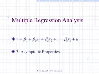
37. Multiple Regression Analysis: Further Issues y = b0 + b1x1 + b2x2 + . . . bkxk + u

38. Functional Form • OLS can be used for relationships that are not strictly linear in x and y by using nonlinear functions of x and y – will still be linear in the parameters • Can take the natural log of x, y or both • Can use quadratic forms of x • Can use interactions of x variable

39. Interpretation of Log Models • If the model is ln(y) = b0 + b1ln(x) + u b1 is the elasticity of y with respect to x • If the model is ln(y) = b0 + b1x + u b1 is approximately the percentage change in y given a 1 unit change in x • If the model is y = b0 + b1ln(x) + u b1 is approximately the change in y for a 100 percent change in x

40. Why use log models? • Log models are invariant to the scale of the variables since measuring percent changes • They give a direct estimate of elasticity • For models with y > 0, the conditional distribution is often heteroskedastic or skewed, while ln(y) is much less so • The distribution of ln(y) is more narrow, limiting the effect of outliers

41. Adjusted R-Squared • Recall that the R2 will always increase as more variables are added to the model • The adjusted R2 takes into account the number of variables in a model, and may decrease

42. Adjusted R-Squared (cont) • It’s easy to see that the adjusted R2 is just (1 – R2)(n – 1) / (n – k – 1), but most packages will give you both R2 and adj-R2 • You can compare the fit of 2 models (with the same y) by comparing the adj-R2 • You cannot use the adj-R2 to compare models with different y’s (e.g. y vs. ln(y))

43. The Use and Interpretation of the Constant Term General Rule • Do Not Suppress the Constant Term ( Even if theory specifically calls for it ) • Do Not Rely on estimates of the Constant Term

44. Multiple Regression Assumptions • 1. a. Linearity: The relationship between dependent and independent variables is linear • Just like bivariate regression • Points don’t all have to fall exactly on the line; but error (disturbance) must be random • Check scatterplots of X’s and error (residual) • Watch out for non-linear trends: error is systematically negative (or positive) for certain ranges of X • There are strategies to cope with non-linearity, such as including X and X-squared to model curved relationship.

45. Multiple Regression Assumptions • 1. b. And, the model is properly specified: • No extra variables are included in the model, and no important variables are omitted. This is HARD! • Correct model specification is critical • If an important variable is left out of the model, results are biased (“omitted variable bias”) • Example: If we model job prestige as a function of family wealth, but do not include education • Coefficient estimate for wealth would be biased • Use theory and previous research to decide what critical variables must be included in your model. • For final paper, it is OK if model isn’t perfect.

46. Multiple Regression Assumptions • 2. All variables are measured without error • Unfortunately, error is common in measures • Survey questions can be biased • People give erroneous responses (or lie) • Aggregate statistics (e.g., GDP) can be inaccurate • This assumption is often violated to some extent • We do the best we can: • Design surveys well, use best available data • And, there are advanced methods for dealing with measurement error.

47. Multiple Regression Assumptions • 3. The error term (ei) has certain properties • Recall: error is a cases deviation from the regression line • Not the same as measurement error! • After you run a regression, SPSS can tell you the error value for any or all cases (called the “residual”) • 3. a. Error is conditionally normal • For bivariate, we looked to see if Y was conditionally normal… Here, we look to see if error is normal • Examine “residuals” (ei) for normality at different values of X variables.

48. Regression Assumptions Examine residuals at different values of X. Make histograms and check for normality. Good Not very good • Normality:

49. Multiple Regression Assumptions • 3. b. The error term (ei) has a mean of 0 • This affects the estimate of the constant. (Not a huge problem) • 3. c. The error term (ei) is homoskedastic (has constant variance) • Note: This affects standard error estimates, hypothesis tests • Look at residuals, to see if they spread out with changing values of X • Or plot standardized residuals vs. standardized predicted values.

50. Regression Assumptions Examine error at different values of X. Is it roughly equal? • Homoskedasticity: Equal Error Variance Here, things look pretty good.