Download
1 / 51
510 likes | 632 Vues
This lecture provides a comprehensive summary of emission lines from ionized gas, focusing on Active Galactic Nuclei (AGN) and their historical perspective. It discusses the taxonomy of AGN and the standard model of the black hole paradigm. Essential concepts include the mechanisms of upward and downward transitions in ionized gas, critical densities for line emissions, and methods for measuring gas density and temperature through line ratios. Key references and advanced texts are listed for further reading on AGN, gaseous nebulae, and their characteristic emission lines.

E N D
Lecture: April 3, 2003 • Summary of Emission Lines from Ionized Gas • Introduction to AGN • Historical Perspective • AGN Taxonomy • Standard Model - Black Hole Paradigm
Useful References Gaseous Nebulae: • Shu (pg 216) • Online notes • Osterbrock AGN: • C&O Ch 26 • Introduction toActive Galactic Nuclei by Peterson(first chapter available free online; see reading references on class webpage) • Active Galactic Nuclei by Krolik(more advanced graduate-level textook) • Quasars and Active Galactic Nuclei - An Introduction , by A.K.Kembhavi and J.V.Narlikar (slightly more advanced graduate-level textbook)
In equilibrium, upward transition rate from level 1 balances downard transition rate to level 1 Summary of Emission Lines from Ionized Gas Forbidden Lines from Ionized Gas: “2-Level Atom” 2 E21 1 • Downward transitions can occur through: • Spontaneous decay (rate determined by A21) • collisional de-excitation (elastic collisions with electrons) • Upward transitions can occur through: • photoionization from a lower level • collisional excitation (inelastic collisions with electrons)
[2] This means: Einstein A-coefficient [1] Collisional de-excitation coefficient Increases with ne Increases with n1 Collisional excitation coefficient The collisional coefficients are related through the Boltzmann factor Where g2, g1, are the statistical weights of the two levels (=2J+1)
The collisional de-excitation coefficient is given approximately by: Where the thermal speed of the electrons is given by: And an elastic cross section given approximately by A more detailed calculation yields: Where W12 comes from quantum mechanical calculations
Using Equations [1] and [2], we get that the level populations are related by: [3] The limiting cases are: Boltzmann distr. This defines the critical density for a transition; at densities above the critical density, transitions from the upper to lower level are more likely to occur through collisions rather than spontaneous decay.
How do we use this information? The luminosity of a line (per unit volume) caused by a downward transition from 2 -> 1 is: Using equation [3], this becomes: At low densities: At high densities:
The transition between these two regimes occurs at the critical density: This is a useful diagnostic - if we don't see certain lines of an ion, it may be because the density is too high for their radiation to occur. This happens when the mean time between collisions is comparable to or less than the radiative lifetime A21-1. (This is why we don’t see forbidden lines on Earth) For permitted transitions (electric dipole radiation), the transitions rates occur at A ~ 108 sec-1 and corresponding critical densities of 1015 cm-3. For forbidden lines, the A coefficients are much smaller so the critical densities are much lower - comparable to densities in typical nebulae.
Critical densities for some common transitions: Appenzeller and Östreicher 1988 (AJ 95, 45) and Table 3.11 of Osterbrock Many of these lines are seen in gaseous nebulae, and the strength of the lines depends on the density of the gas
So, summarizing, because these lines are excited primarily by collisions with electrons, the observed line strengths can be used to measure the density, temperature, and then composition of the gas!! To measure density: Use line ratios from lines with different critical densities (but are close together in energy to eliminate temperature dependence ) one in the low-density limit (L a n2) and one in the high-density limit (L a n). In this example, the [SII] at 6716Å comes from a 4S3/2-2D5/2 transition and has a critical density of 1.5 x 103 cm-3. The 6731Å line comes from the 4S3/2-2D3/2 transition with critical density 3.9 x 103 cm-3. Note that the line ratio is sensitivite to density between about 100 to 10,000 cm-3.
To measure temperature: Again use single ion (independent of abundance and ionization) but pick lines that have large differences in excitation potential. The most-used example is [O III] with lines at 4363 and 4959+5007 Å. Once these line ratios are used to constrain density and temperature, abundances can be derived!
The Nature of the Ionizing Source: Since the ions observed are ionized by photons, and the ionization potential of metals varies, line ratios of lines from various ions can be used to infer the spectral shape of the ionizing radiation field. Here are the ionization potentials (eV) for a few common ions: Since even the most massive (hottest) stars produce very few photons beyond ~ 50 eV, the presence of lines from highly ionized species indicated the presence of some source of hard photons other than stars. What could this be? Next topic:AGN
Introduction to Active Galactic Nulcei (AGN) • Historical Background • Taxonomy - Classes of AGN • Brief overview of continuum and spectral characteristics
Denition What are Active Galactic Nuclei? Active Galactic Nuclei (AGN) are nuclei of galaxies which show energetic phenomena that cannot be clearly and directly attributed to stars. Signs of Activity: • Luminous UV emission from a compact region in the center of a galaxy • Strongly Doppler-broadened emission lines • High variability • Strong non-thermal emission ; polarized emission • Compact radio core • Extended, linear radio structures (jets+hotspots) • X-ray, g-ray, and TeV-emission In some luminous AGN (quasars) the radiation from a region comparable to the solar system can be several hundred times brighter than the whole galaxy.
Historical Perspective • First detections • NGC 1068 (E.A. Fath 1908, Lick Obs.) and V.M. Slipher (Lowell Obs.) - strong emission lines similar to planetary nebulae, line widths of several hundred km/sec • Detection of an optical jet in M87 (Curtis 1913) • Same period: Einstein develops GR, Schwarzschild metric (1916), but no connection seen yet • Hubble (1926) - Nebulae are extragalactic (galaxies) • Carl Seyfert (1943) - found several galaxies similar to NGC1068 (henceforth named Seyfert galaxies), i.e. galxies with a bright nucleus and strong emission lines (NGC1275, NGC3516, NGC 4051, NGC 4151, NGC7469) • Detection of radio emission from NGC1068 & NGC1275 (1955) • Woltjer (1959) - Timescale for Seyfert-activity 108 years (1% of Galaxies are luminous Seyferts), Mass of nucleus is very high 108-10 M(velocity dispersion/line width several thousandkm/sec at base in unresolved nucleus)
Historical Perspective Radio Surveys & Quasars • Early radio surveys were very important for the discovery of quasars. For example: • 3C and 3CR: The third Cambridge (3C) catalog (Edge et • al. 1959) at 158 MHz. Revision: 3CR catalog (Bennett 1961) • at 178 MHz down to limiting flux density of 9 Jy (1 Jy = 10-26 W m-2 Hz-1) - Discovery of first quasars (e.g. 3C273,279) • PKS: Parkes (Australia, Ekers 1969) survey of southern sky at • 408 MHz (> 4 Jy) and 1410 MHz (> 1 Jy). • Sources found: • Normal Galaxies • Stars with weird broad emission lines!?
Detection of Quasars Radio ID of quasars by Hazard et al. (1963), Maarten Schmidt (1963): The lines in 3C273 are highly redshifted (z=0.158) emission lines ! first detection of quasars (3C 48, 3C273), from Hubbles law follows (h0 = H0/(100 km s-1 Mpc-1) (100 times larger than normal galaxy) quasar = quasi-stellar radio source, QSO = quasi-stellar object (no longer distinguished)
AGN were quickly seen to show emission in all astrophysically relevant wavelengths regimes
AGN Taxonomy • Seyfert galaxies 1 and 2 • Quasars (QSOs and QSRs) • Radio Galaxies • LINERs • Blazars • Related phenomena
Seyferts • Lower-luminosity AGN MB > -21.5 + 5log(H0/100) (Schmidt & Green 1983) • Quasar-like nucleus; host galaxy clearly seen • Seyferts occur mainly in spirals • Nucleus has strong, high-ionization emission lines in the optical
Optical spectra of Seyferts • Broad lines: FWHM~500-10,000 km/s permitted lines; high-density gas (ne> 109 cm-3) ~ pc distance from center • Narrow lines: FWHM ~ hundreds km/s forbidden lines low-density gas (ne~ 103-6 cm-3) ~ 50-100 pc distance • Absorption features due to stars in the host galaxy
BLR/NLR Diagnostic • Dynamics gives clouds location • Types of lines observed/not observed give info on temperature, density Example: [OIII] λ5007 not observed from BLR critical de-excitation density ne~106cm-3 lower limit [CIII]λ1909 is observed from BLR critical de-excitation density ne~1010cm-3 upper limit
Seyferts 1 and 2 • Seyferts 1: both broad and narrow lines Balmer lines, [OIII] λ4959,5007 • Seyferts 2: only narrow lines [OIII] λ4959,5007 • Intermediate types: 1.1-1.9 decreasing intensity of the broad line component
Reddened continuum Seyfert 2 LINER
Quasars • Most luminous AGN MB< -21.5 + 5log(H0/100) • Unresolved (<7”) on Palomar Plates • Weak “fuzz” on deep observations (HST) • Similar nuclear spectra to Seyferts, but weaker abs lines and narrow/broad ratios QSO=optically bright (most) QSR=radio bright (5-10%)
Radio Galaxies • Occur in giant ellipticals • Bright radio emission with extended features (jets, lobes) and compact core • Broad-Line Radio Galaxies (BLRGs) Narrow-Line Radio Galaxies (NLRGs) QSRs
LINERs • Low Ionization Nuclear Emission Lines • Very faint, and numerous; may be ~50% of local extragalactic population • Similar to Sy2 but stronger low-ionization lines • What are LINERs? Ratios of line fluxes depends on shape of ionizing continuum
Starlight vs AGN light • Ionization potential for O to OIII: 54.93 eV • AGN produce many photons at these energies Are LINERs powered by faint AGN?
LINER diagnostic Ho et al. 1989 x=HII regions LINERs Seyferts
Blazars • High luminosity, non-thermal continuum from radio to gamma-rays • Flat or inverted radio spectrum • Rapid variability T day- hours • Large Polarizations ~ 10% BL Lacs: weak emission lines, nearby OVVs/FSRQs: strong emission lines, distant
Related Phenomena • Starbursts: Intense starformation, often nuclear bright in optical, X-rays, radio • Markarian galaxies: from Markarian survey at Byurakan Observatory, Armenia UV-excess galaxies 11% Seyferts, 2% QSOs and BL Lacs • ULIRGs:from IRAS survey in the 80s at λ>10μ L(8-1000μ) > 1012Lsolar due to dust heated by AGN/Starburst
What powers AGN? • It is very difficult to explain the observed set of characteristics of AGN without invoking a supermassive central black hole.
AGN: What are they good for? • Study black hole physics • Study high energy physics • Background sources on cosmological scales: • -Ly-a forrest in optical spectra (absorbing gas in cosmic walls?) • -Are gravitationally lensed by clusters, get Hubble constant from time delay • -Background radiation to detect absorption lines in host galaxies at large z • -Produce cosmic background radiation, e.g. at X-ray wavelengths • Find galaxies at highest redshifts (z > 5.8!) • Constrain cosmology • History of our Galaxy; impact on galaxy evolution
The Black Hole Paradigm Basic question early on: what powers quasars, Seyferts, and radio galaxies? Remember: the characteristic signatures of quasars are • high luminosity (L > 1044 erg/sec, i.e. 1010.5-14.5 L) • high compactness (variability on time scales of years, compact • radio cores < 1pc) Such a high luminosity will produce an enormous radiation pressure. Hence, for material to be gravitational bound to the center of the galaxy, we can calculate a minimum central mass - the Eddington mass - independent of a particular model.
Eddington Limit • The momentum of photons is l = E/c (one photon: E =hn) • the force F of photons is F = dl/dt = E/c • the pressure is force per area P = F/A Hence, the radiation pressure at distance r of an isotropically radi- ating point source of luminosity L is (L: luminosity, F: flux density) The force exerted on a single electron is obtained by multiplying with the electron scattering cross-section (dimension cm2):
Here se is the Thomson cross-section (from classical electron radius) The inward directed gravitational force of a central mass M is given by NB: The radiation pressure is mainly acting on the electrons while gravitation mainly acts on protons (since they have bigger mass). Coulomb forces will keep them together! In order for matter to be gravitationally bound (to fall inward), we need which is independent of the radius.
This condition is called the Eddington Limit and states that fora given luminosity a certain minimum central mass is required (Eddington mass) or that for a given central mass the luminosity cannot exceed the Eddington luminosity.
Schwarzchild Radius Equating kinetic and potential energy in a gravitating system yields: setting v = c-the speed of photons-and canceling m we get: This is called the Schwarzschild radius and defines the event horizon in the Schwarzschild metric (non-rotating black hole). • For the mass of the earth we have RS= 1cm • For a quasar with M = 108 M we have RS = 3 x 1013 cm = 2 AU.
When mass falls onto a black hole, potential energy is converted into kinetic energy. This energy is either advected into and beyond the event horizon or released before. The potential energy of a mass element dm in a gravitational field is The available energy (luminosity) then is where we call the mass accretion rate The characteristic scale of the emitting region will be a few gravitational radii, i.e. r ~ rinRs
Efficiency is just a function of how compact the object is The compactness of the accretion disk will depend on the spin (a) of the black hole: for a = 0 (Schwarzschild) we have = 6% and for a = 1 (extreme Kerr) we have = 40%! Note that for nuclear fusion we only have = 0.007. For a quasar with L=1046 ergs/s and =0.1, we have M = 2 M yr-1. Accretion is the most efficient energy-generation process currently known
Where does the luminosity come from? Accretion Disks Luminosity of AGN derives from gravitational potential energy of gas spiraling inward through an accretion disk. Mass streams are in orbit around the BH; viscosity, an internal force that converts the directed KE of the bulk mass motion into random thermal motion, causes orbiting gas to lose angular momentum and fall inwards. Energy is dissipated in the disk and is radiated away.
Angular momentum transport If the disk is thin (this means that the orbital velocity is much greater than the sound speed), then orbital velocity of the gas is Keplerian: Specific angular momentum vfR is: i.e. increasing outwards. Gas at large R has too much angular momentum to be accreted by the black hole. To flow inwards, gas must lose angular momentum, either: • By redistributing the angular momentum within the disk (gas at small R loses angular momentum to gas further out and flows inward) • By loss of angular momentum from the entire system.e.g. a wind from the disk could take away angular momentum allowing inflow
Redistribution of angular momentum within a thin disk is a diffusive process - a narrow ring of gas spreads out under the action of the disk viscosity: Gas surface density Radius, R With increasing time: • Mass all flows inward to small R and is accreted • Angular momentum is carried out to very large R by a vanishingly small fraction of the mass
Radiation from thin disk accretion Consider gas flowing inward through a thin disk. Easy to estimate the radial distribution of temperature. The total energy felt by a mass m of orbiting gas is: Conservation of energy required that energy dE radiated in time t be equal to energy difference between the two boundaries in picture above: R-dR R If the luminosity of the ring is dLring, then: Using Stefan-Boltzmann law with A=2(2prdr): Solving for T:
Correct dependence on mass, accretion rate, and radius, but wrong prefactor. Need to account for: • Radial energy flux through the disk (transport of angular momentum also means transport of energy) • Boundary conditions at the inner edge of the disk Correcting for this, radial distribution of temperature is: †…where Rin is the radius of the disk inner edge. For large radii R >> Rin, we can simplify the expression to: with Rs the Schwarzschild radius as before. For a hole accreting at the Eddington limit: • Accretion rate scales linearly with mass • Schwarzschild radius also increases linearly with mass Temperature at fixed number of Rs decreases as M-1/4 Disks around more massive black holes are cooler.
For a supermassive black hole, rewrite the temperature as: Accretion rate at the Eddington limiting luminosity (assuming h=0.1) A thermal spectrum at temperature T peaks at a frequency: An inner disk temperature of ~105 K corresponds to strong emission at frequencies of ~1016 Hz. Wavelength ~50 nm. Expect disk emission in AGN accreting at close to the Eddington limit to be strong in the ultraviolet – origin of the broad peak in quasar SEDs in the blue and UV.