Process Control Instrumentation II
520 likes | 1.07k Vues
Process Control Instrumentation II. Module 2. Module 2.

Process Control Instrumentation II
E N D
Presentation Transcript
Process Control Instrumentation II Module 2
Module 2 • Optimum controller settings : Evaluation criteria – IAE, ISE, ITAE and ¼ decay ratio – determination of optimum settings for mathematically described processes using time response and frequency response – tuning – Process Reaction Curve method – Ziegler Nichols method – Damped oscillation method.
Evaluation Criteria • To define What is a GOOD control, which may differ from process to process. • How to Select the type of feedback controller – P, PI, PD or PID • How to adjust parameters – Kp, KI, KD We can: • Keep the maximum deviation (error) as small as possible. • Achieve short settling times. • Minimize the Integral of errors until the process has settled to its desired set point.
Performance Criteria If the criterion is to ‘return to desired value as soon as possible’, then we select closed loop response ‘A’. If the criterion is to ‘keep the maximum deviation as small as possible’ we select response ‘B’.
Performance Criteria • Steady State Performance Criteria • Dynamic Response Performance Criteria Steady State Performance Criteria - ‘Zero error at steady state’ • Proportional controller cannot achieve zero error due to offset, but PI mode can. • For a Proportional control steady state error tends to zero when Kp→∞
Performance Criteria Dynamic Response Performance Criteria based on two criteria: • Simple Performance Criteria: • uses only a few points of the response. • They are simpler, but only approximate. • Time Integral Performance Criteria: • uses entire closed loop response from t=0 to t= very large. • They are precise, but difficult to use.
Simple Performance Criteria • Different parameters like Overshoot, rise time, settling time, decay ratio and frequency of oscillation of the transient are considered. • Most popular is DECAY RATIO criterion.
One Quarter Decay Ratio Criterion The measure of decay ratio is found by adjusting the control loop until the deviation from the disturbance is such that each deviation peak is down by one quarter from the preceding peak.
Time Integral Performance Criteria • The shape of complete closed loop response from time t=0 until steady state reached is used. • It uses the entire response, but in the case of ¼ ratio criteria it uses only isolated characteristics of the dynamic response. • It is more precise. • In ¼ ratio criteria many combinations of controller settings are possible; but in integral criteria only one combination is possible which certainly reduces the error.
Time Integral Performance Criteria Integral of the Square Error (ISE) ISE criteria give more weight to larger deviations
Time Integral Performance Criteria 2. Integral of the Absolute value of Error (IAE) It seems the best criterion for process control, since the penalty for control is generally a linear function of the error.
Time Integral Performance Criteria 3. Integral of the Time weighted Absolute Error (ITAE) ITAE criteria weights deviations more heavily as time increases.
Time Integral Performance Criteria • If we want to suppress large errors, ISE is better than IAE, because the errors are squared and thus contribute more to the value of integral. • For the suppression of small errors, IAE is better than ISE because when we square small errors they become even smaller. • To suppress errors that persists for longer times, ITAE criterion is better because of the presence of ‘t’ in the integral term.
Time Integral Performance Criteria • Different criteria lead to different controller designs. • For the same time integral criterion, different input changes lead to different designs.
Selection of Feedback Controller Define an appropriate performance criterion (ISE, IAE or ITAE) Compute the value of the performance criterion using a P or PI or PID controller with the best settings for the adjusted parameters KP, KI and KD Select the controller which gives the ‘best’ value for the performance criterion.
Proportional Control Accelerates the response of a controlled process. Produces an offset. • Integral Control Eliminates any offset. Higher maximum deviation. Produces sluggish, long oscillating response. If we increase KP to produce faster response, the system become oscillatory and may lead to instability.
Derivative Control Anticipates future errors and introduces appropriate action. Introduces a stabilizing effect on the closed-loop response of a process.
Process of deciding what values to be used for its adjusted parameters for a feed back controller. 3 General approaches for controller tuning: Use simple criteria such as ¼ decay ratio, minimum settling time, minimum largest error and so on. (Since it provides multiple solutions, additional specifications needed to be considered to reach a single solution and new value to parameters) Use time integral performance criteria (IAE, ISE, ITAE). (it is cumbersome and relies heavily on mathematical model. If applied experimentally on actual process it is time consuming.) Use Semi empirical rules which have been proven in practice. CONTROLLER TUNING
PROCESS REACTION CURVE METHOD(Cohen and Coon Method) • Also called OPEN LOOP TRANSIENT RESPONSE METHOD. • Opening the control loop by disconnecting the controller output from the final control element. • Can be used only for systems with ‘self regulation’.
PROCESS REACTION CURVE METHOD • Open the control loop by disconnecting the controller output from the final control element. • Introduce a step change of magnitude ‘A’ in the variable ‘c’ which actuates FCE. • Record the value of output with respect to time. This curve ym(t) is called ‘PROCESS REACTION CURVE’.
PROCESS REACTION CURVE METHOD • PRC is affected by the dynamics of process, sensor and FCE. • Cohen and Coon observed a ‘sigmoidal shape’ which can be approximated to a first order system with a dead time.
PROCESS REACTION CURVE METHOD Static Gain Time constant = slope of the sigmoidal response at the point of inflection. Dead time td = time elapsed until the system responded • Derive expressions for the best controller settings
PROCESS REACTION CURVE METHOD Proportional Controller
PROCESS REACTION CURVE METHOD Proportional – Integral Controller
PROCESS REACTION CURVE METHOD Proportional - Integral - Derivative Controller
PROCESS REACTION CURVE METHOD • Observations: • Gain of PI controller is less than P controller because integral mode makes the system more sensitive (oscillatory). • The stabilizing effect of derivative control mode allows the use of higher gains in PID controller compared to P and PI controllers.
ZIEGLER-NICHOLS METHOD(Ultimate Cycling Method) • Also called CLOSED LOOP TUNING METHOD. • This method based on frequency response analysis. • Adjusting closed loop until steady oscillations occur, controller settings are then based on the conditions that generate the cycling.
ZIEGLER-NICHOLS METHOD Bring the system to desired operational level (Design condition). Reduce any Integral and derivative action to their minimum effect. Using proportional control only and with feedback loop closed, introduce a set point change and vary proportional gain until the system oscillates continuously. The frequency of continuous oscillations is the cross over frequency, ‘ω0’. Let ‘M’ be the amplitude ratio of the system’s response at the cross over frequency.
ZIEGLER-NICHOLS METHOD Compute the following two quantities: Ultimate Gain KU= 1/M Ultimate period of sustaining cycling, PU = 2π/ωCOmin/ cycle 5. Using the values of KU and PU compute controller settings.
DAMPED OSCILLATION METHOD • Sustained oscillations for testing purpose are not allowable in many plants. So Ziegler- Nichols Method cannot be used. • More accurate than Closed loop method • By using only proportional action and starting with a low gain, the gain is adjusted until the transient response of the closed loop shows a decay ratio of ¼. • The reset time and derivative time are based on the period of oscillation, P, which is always greater than the ultimate period PU.
DAMPED OSCILLATION METHOD For PID control TD = P/6 TI = P/1.5