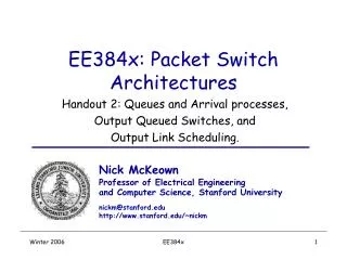
EE384x: Packet Switch Architectures
EE384x: Packet Switch Architectures. Handout 2: Queues and Arrival processes, Output Queued Switches, and Output Link Scheduling. Nick McKeown Professor of Electrical Engineering and Computer Science, Stanford University nickm@stanford.edu http://www.stanford.edu/~nickm. Outline.

EE384x: Packet Switch Architectures
E N D
Presentation Transcript
EE384x: Packet Switch Architectures Handout 2: Queues and Arrival processes, Output Queued Switches, and Output Link Scheduling. Nick McKeown Professor of Electrical Engineering and Computer Science, Stanford University nickm@stanford.edu http://www.stanford.edu/~nickm EE384x
Outline • Output Queued Switches • Terminology: Queues and arrival processes. • Output Link Scheduling EE384x
Data Data Data Hdr Hdr Hdr Header Processing Header Processing Header Processing Lookup IP Address Lookup IP Address Lookup IP Address Update Header Update Header Update Header Address Table Address Table Address Table N times line rate Generic Router Architecture 1 1 Queue Packet Buffer Memory 2 2 Queue Packet Buffer Memory N times line rate N N Queue Packet Buffer Memory EE384x
Link 1, ingress Link 1, egress Link 2, ingress Link 2, egress Link 3, ingress Link 3, egress Link 4, ingress Link 4, egress Simple model of output queued switch Link rate, R Link rate, R Link 2 Link 1 R1 Link 3 R R Link 4 R R R R EE384x
Characteristics of an output queued (OQ) switch • Arriving packets are immediately written into the output queue, without intermediate buffering. • The flow of packets to one output does not affect the flow to another output. • An OQ switch is work conserving: an output line is always busy when there is a packet in the switch for it. • OQ switch have the highest throughput, and lowest average delay. • We will also see that the rate of individual flows, and the delay of packets can be controlled. EE384x
The shared memory switch A single, physical memory device Link 1, ingress Link 1, egress Link 2, ingress Link 2, egress R R Link 3, ingress Link 3, egress R R Link N, ingress Link N, egress R R EE384x
Memory bandwidth Basic OQ switch: • Consider an OQ switch with N different physical memories, and all links operating at rate R bits/s. • In the worst case, packets may arrive continuously from all inputs, destined to just one output. • Maximum memory bandwidth requirement for each memory is (N+1)R bits/s. Shared Memory Switch: • Maximum memory bandwidth requirement for the memory is 2NR bits/s. EE384x
How fast can we make a centralized shared memory switch? 5ns SRAM Shared Memory • 5ns per memory operation • Two memory operations per packet • Therefore, up to 160Gb/s • In practice, closer to 80Gb/s 1 2 N 200 byte bus EE384x
Outline • Output Queued Switches • Terminology: Queues and arrival processes. • Output Link Scheduling EE384x
Queue Terminology A(t), l D(t) S,m • Arrival process, A(t): • In continuous time, usually the cumulative number of arrivals in [0,t], • In discrete time, usually an indicator function as to whether or not an arrival occurred at time t=nT. • l is the arrival rate; the expected number of arriving packets (or bits) per second. • Queue occupancy, Q(t): • Number of packets (or bits) in queue at time t. • Service discipline, S: • Indicates the sequence of departure: e.g. FIFO/FCFS, LIFO, … • Service distribution: • Indicates the time taken to process each packet: e.g. deterministic, exponentially distributed service time. • m is the service rate; the expected number of served packets (or bits) per second. • Departure process, D(t): • In continuous time, usually the cumulative number of departures in [0,t], • In discrete time, usually an indicator function as to whether or not a departure occurred at time t=nT. Q(t) EE384x
More terminology • Customer: queueing theory usually refers to queued entities as “customers”. In class, customers will usually be packets or bits. • Work: each customer is assumed to bring some work which affects its service time. For example, packets may have different lengths, and their service time might be a function of their length. • Waiting time: time that a customer waits in the queue before beginning service. • Delay: time from when a customer arrives until it has departed. EE384x
Arrival Processes • Examples of deterministic arrival processes: • E.g. 1 arrival every second; or a burst of 4 packets every other second. • A deterministic sequence may be designed to be adversarial to expose some weakness of the system. • Examples of random arrival processes: • (Discrete time) Bernoulli i.i.d. arrival process: • Let A(t) = 1 if an arrival occurs at time t, where t = nT, n=0,1,… • A(t) = 1 w.p. pand 0 w.p.1-p. • Series of independent coin tosses with p-coin. • (Continuous time) Poisson arrival process: • Exponentially distributed interarrival times. EE384x
Adversarial Arrival ProcessExample for “Knockout” Switch Memory write bandwidth = k.R< N.R 1 R R If our design goal was to not drop packets, then a simple discrete time adversarial arrival process is one in which: • A1(t) = A2(t) = … = Ak+1(t) = 1, and • All packets are destined to output t mod N. 2 R R 3 R R N R R EE384x
Bernoulli arrival process Memory write bandwidth = N.R 1 A1(t) R R 2 A2(t) R R 3 A3(t) R R N AN(t) R R • Assume Ai(t) = 1 w.p. p, else 0. • Assume each arrival picks an output independently, uniformly and at random. • Some simple results follow: • 1. Probability that at time t a packet arrives to input i destined to output j is p/N. • 2. Probability that two consecutive packets arrive to input i is the same as the probability that packets arriveto inputs i and j simultaneously, equals p2. • Questions: • 1. What is the probability that two arrivals occur at input i in any three time slots? • 2. What is the probability that two arrivals occur for output j in any three time slots? • 3. What is the probability that queue i holds k packets? EE384x
Simple deterministic model Cumulative number of bits that arrived up until time t. A(t) A(t) Cumulative number of bits D(t) Q(t) R Service process time D(t) • Properties ofA(t), D(t): • A(t), D(t) are non-decreasing • A(t) >= D(t) Cumulative number of departed bits up until time t. EE384x
Simple Deterministic Model Cumulative number of bits d(t) A(t) Q(t) D(t) time Queue occupancy: Q(t) = A(t) - D(t). Queueing delay, d(t), is the time spent in the queue by a bit that arrived at time t, (assuming that the queue is served FCFS/FIFO). EE384x
Outline • Output Queued Switches • Terminology: Queues and arrival processes. • Output Link Scheduling EE384x
The problems caused by FIFO queues in routers • In order to maximize its chances of success, a source has an incentive to maximize the rate at which it transmits. • (Related to #1) When many flows pass through it, a FIFO queue is “unfair” – it favors the most greedy flow. • It is hard to control the delay of packets through a network of FIFO queues. Fairness Delay Guarantees EE384x
Fairness 10 Mb/s 0.55 Mb/s A 1.1 Mb/s 100 Mb/s C R1 e.g. an http flow with a given (IP SA, IP DA, TCP SP, TCP DP) 0.55 Mb/s B What is the “fair” allocation: (0.55Mb/s, 0.55Mb/s) or (0.1Mb/s, 1Mb/s)? EE384x
Fairness 10 Mb/s A 1.1 Mb/s R1 100 Mb/s D B 0.2 Mb/s What is the “fair” allocation? C EE384x
Max-Min FairnessA common way to allocate flows N flows share a link of rate C. Flow f wishes to send at rate W(f), and is allocated rate R(f). • Pick the flow, f, with the smallest requested rate. • If W(f)< C/N, then set R(f) = W(f). • If W(f) > C/N, then set R(f) = C/N. • Set N = N – 1. C = C – R(f). • If N>0 goto 1. EE384x
Max-Min FairnessAn example W(f1) = 0.1 1 Round 1: Set R(f1) = 0.1 Round 2: Set R(f2) = 0.9/3 = 0.3 Round 3: Set R(f4) = 0.6/2 = 0.3 Round 4: Set R(f3) = 0.3/1 = 0.3 W(f2) = 0.5 C R1 W(f3) = 10 W(f4) = 5 EE384x
Max-Min Fairness • How can an Internet router “allocate” different rates to different flows? • First, let’s see how a router can allocate the “same” rate to different flows… EE384x
Fair Queueing • Packets belonging to a flow are placed in a FIFO. This is called “per-flow queueing”. • FIFOs are scheduled one bit at a time, in a round-robin fashion. • This is called Bit-by-Bit Fair Queueing. Flow 1 Bit-by-bit round robin Classification Scheduling Flow N EE384x
Weighted Bit-by-Bit Fair Queueing Likewise, flows can be allocated different rates by servicing a different number of bits for each flow during each round. R(f1) = 0.1 1 R(f2) = 0.3 C R1 R(f3) = 0.3 R(f4) = 0.3 Order of service for the four queues: … f1, f2, f2, f2, f3, f3, f3, f4, f4, f4, f1,… Also called “Generalized Processor Sharing (GPS)” EE384x
Packetized Weighted Fair Queueing (WFQ) Problem: We need to serve a whole packet at a time. Solution: • Determine what time a packet, p, would complete if we served flows bit-by-bit. Call this the packet’s finishing time, F. • Serve packets in the order of increasing finishing time. Theorem: Packet p will depart before F + TRANSPmax Also called “Packetized Generalized Processor Sharing (PGPS)” EE384x
Calculating F • Assume that at time t there are N(t) active (non-empty) queues. • Let R(t) be the number of rounds in a round-robin service discipline of the active queues, in [0,t]. • A P bit long packet entering service at t0 will complete service in round R(t) = R(t0) + P. EE384x
Case 1: If packet arrives to non-empty queue, then Si = Fi-1 Case 2: If packet arrives at t0 to empty queue, then Si = R(t0) An example of calculating F Flow 1 R(t) Flow i Pick packet with smallest Fi & Send Calculate Si and Fi & Enqueue Flow N • In both cases, Fi = Si + Pi • R(t) is monotonically increasing with t, therefore • same departure order in R(t) as in t. EE384x
6 5 4 3 2 1 0 Time A1 = 4 1 1 1 1 1 1 1 1 1 1 1 1 B1 = 3 C2 = 1 C1 = 1 D1 = 1 D2 = 2 Weights : 1:1:1:1 6 5 4 3 2 1 0 D1, C1 Depart at R=1 Time A2, C3 arrive A2 = 2 A1 = 4 D1 C1 B1 A1 B1 = 3 C3 = 2 C2 = 1 C1 = 1 Round 1 D1 = 1 D2 = 2 Weights : 1:1:1:1 6 5 4 3 2 1 0 Time C2 Departs at R=2 A2 = 2 A1 = 4 D2 C2 B1 A1 D1 C1 B1 A1 B1 = 3 C3 = 2 C2 = 1 C1 = 1 Round 2 Round 1 D1 = 1 D2 = 2 Weights : 1:1:1:1 Understanding bit by bit WFQ 4 queues, sharing 4 bits/sec of bandwidth, Equal Weights EE384x
6 5 4 3 2 1 0 Time D2, B1 Depart at R=3 A2 = 2 A1 = 4 1 1 1 1 1 1 1 1 1 1 1 1 D2 C2 B1 A1 D2 C3 B1 A1 D1 C1 B1 A1 B1 = 3 C3 = 2 C2 = 1 C1 = 1 D1 = 1 D2 = 2 6 5 4 3 2 1 0 A2 Departs at R=6 C3, A1 Depart at R=4 Weights : 1:1:1:1 Time A2 = 2 A1 = 4 D2 C2 B1 A1 A2 A2 C3 A1 D2 C3 B1 A1 D1 C1 B1 A1 B1 = 3 C3 = 2 C2 = 1 C1 = 1 6 5 Round 4 Round 3 D1 = 1 D2 = 2 Sort packets Weights : 1:1:1:1 Time 6 5 4 3 2 1 0 Departure order for packet by packet WFQ: Sort by finish round of packets A2 = 2 A1 = 4 A2 A2 C3 C3 A 1 A 1 A1 A 1 D2 D2 B1 B1 B1 C2 D1 C1 B1 = 3 Round 2 Round 2 Round 1 Round 1 C3 = 2 C2 = 1 C1 = 1 D1 = 1 D2 = 2 Weights : 1:1:1:1 Understanding bit by bit WFQ 4 queues, sharing 4 bits/sec of bandwidth, Equal Weights Round 3 EE384x
6 5 4 3 2 1 0 Time A1 = 4 3 3 3 2 2 2 2 2 2 1 1 1 B1 = 3 C2 = 1 C1 = 1 D1 = 1 D2 = 2 Weights : 3:2:2:1 6 5 4 3 2 1 0 Time A2 = 2 A1 = 4 B1 A1 A1 A1 B1 = 3 C3 = 2 C2 = 1 C1 = 1 Round 1 D1 = 1 D2 = 2 Weights : 3:2:2:1 6 5 4 3 2 1 0 Time D1, C2, C1 Depart at R=1 A2 = 2 A1 = 4 D1 C2 C1 B1 B1 A1 A1 A1 B1 = 3 C3 = 2 C2 = 1 C1 = 1 Round 1 D1 = 1 D2 = 2 Weights : 3:2:2:1 Understanding bit by bit WFQ 4 queues, sharing 4 bits/sec of bandwidth, Weights 3:2:2:1 EE384x
6 5 4 3 2 1 0 Time B1, A2 A1 Depart at R=2 A2 = 2 A1 = 4 3 3 3 2 2 2 2 2 2 1 1 1 B1 A2 A2 A1 D1 C2 C1 B1 B1 A1 A1 A1 B1 = 3 C3 = 2 C2 = 1 C1 = 1 D1 = 1 D2 = 2 Weights : 3:2:2:1 6 5 4 3 2 1 0 D2, C3 Depart at R=2 Time A2 = 2 A1 = 4 D2 D2 C3 C3 B1 A2 A2 A1 D1 C2 C1 B1 B1 A1 A1 A1 B1 = 3 C3 = 2 C2 = 1 C1 = 1 3 Round 2 Round 1 D1 = 1 D2 = 2 Sort packets Weights : 3:2:2:1 6 5 4 3 2 1 0 Time Departure order for packet by packet WFQ: Sort by finish time of packets A2 = 2 A1 = 4 D2 D2 C3 C3 B1 B 1 B1 A2 A2 A1 A1 A1 A1 D1 C2 C1 B1 = 3 C3 = 2 C2 = 1 C1 = 1 D1 = 1 D2 = 2 Weights : 3:2:2:1 Understanding bit by bit WFQ 4 queues, sharing 4 bits/sec of bandwidth, Weights 3:2:2:1 Round 2 Round 1 Weights : 1:1:1:1 EE384x
WFQ is complex • There may be hundreds to millions of flows; the linecard needs to manage a FIFO per flow. • The finishing time must be calculated for each arriving packet, • Packets must be sorted by their departure time. Naively, with m packets, the sorting time is O(logm). • In practice, this can be made to be O(logN), for N active flows: 1 Egress linecard 2 Calculate Fp Find Smallest Fp Departing packet Packets arriving to egress linecard 3 N EE384x
Step 2,3,4: Active packet queues 100 100 100 600 200 400 400 150 150 600 50 200 340 60 400 Deficit Round Robin (DRR) [Shreedhar & Varghese, ’95]An O(1) approximation to WFQ Step 1: Active packet queues 200 100 100 600 0 400 400 0 150 600 50 0 340 60 400 Quantum Size = 200 • It appears that DRR emulates bit-by-bit FQ, with a larger “bit”. • So, if the quantum size is 1 bit, does it equal FQ? (No). • It is easy to implement Weighted DRR using a different quantumsize for each queue. EE384x
The problems caused by FIFO queues in routers • In order to maximize its chances of success, a source has an incentive to maximize the rate at which it transmits. • (Related to #1) When many flows pass through it, a FIFO queue is “unfair” – it favors the most greedy flow. • It is hard to control the delay of packets through a network of FIFO queues. Fairness Delay Guarantees EE384x
Deterministic analysis of a router queue FIFO delay, d(t) Cumulative bytes Model of router queue A(t) D(t) A(t) D(t) m Q(t) Q(t) m time EE384x
So how can we control the delay of packets? Assume continuous time, bit-by-bit flows for a moment… • Let’s say we know the arrival process, Af(t), of flow f to a router. • Let’s say we know the rate, R(f) that is allocated to flow f. • Then, in the usual way, we can determine the delay of packets in f, and the buffer occupancy. EE384x
Flow 1 R(f1), D1(t) A1(t) Classification WFQ Scheduler Flow N AN(t) R(fN), DN(t) Cumulative bytes Key idea: In general, we don’t know the arrival process. So let’s constrain it. A1(t) D1(t) R(f1) time EE384x
Let’s say we can bound the arrival process r Cumulative bytes Number of bytes that can arrive in any period of length t is bounded by: This is called “(s,r) regulation” A1(t) s time EE384x
dmax Bmax (s,r) Constrained Arrivals and Minimum Service Rate Cumulative bytes A1(t) D1(t) r s R(f1) time Theorem [Parekh,Gallager ’93]: If flows are leaky-bucket constrained,and routers use WFQ, then end-to-end delay guarantees are possible. EE384x
The leaky bucket “(s,r)” regulator Tokens at rate,r Token bucket size,s Packets Packets One byte (or packet) per token Packet buffer EE384x
How the user/flow can conform to the (s,r) regulationLeaky bucket as a “shaper” Tokens at rate,r Token bucket sizes To network Variable bit-rate compression C r bytes bytes bytes time time time EE384x
Checking up on the user/flowLeaky bucket as a “policer” Router Tokens at rate,r Token bucket sizes From network C r bytes bytes time time EE384x
Policer Policer Classifier Classifier Policer Policer QoS Router Per-flow Queue Scheduler Per-flow Queue Per-flow Queue Scheduler Per-flow Queue • Remember: These results assume that it is an OQ switch! • Why? • What happens if it is not? EE384x
References • Abhay K. Parekh and R. Gallager“A Generalized Processor Sharing Approach to Flow Control in Integrated Services Networks: The Single Node Case” IEEE Transactions on Networking, June 1993. • M. Shreedhar and G. Varghese“Efficient Fair Queueing using Deficit Round Robin”, ACM Sigcomm, 1995. EE384x