State Space Analysis
State Space Analysis. UNIT-V. outline. How to find mathematical model, called a state-space representation, for a linear, time-invariant system How to convert between transfer function and state space models. State-Space Modeling. Alternative method of modeling a system than

State Space Analysis
E N D
Presentation Transcript
State Space Analysis UNIT-V
outline • How to find mathematical model, called a state-space representation, for a linear, time-invariant system • How to convert between transfer function and state space models
State-Space Modeling • Alternative method of modeling a system than • Differential / difference equations • Transfer functions • Uses matrices and vectors to represent the system parameters and variables • In control engineering, a state space representation is a mathematical model of a physical system as a set of input, output and state variables related by first-order differential equations. To abstract from the number of inputs, outputs and states, the variables are expressed as vectors.
Motivation for State-Space Modeling • Easier for computers to perform matrix algebra • e.g. MATLAB does all computations as matrix math • Handles multiple inputs and outputs • Provides more information about the system • Provides knowledge of internal variables (states) • Primarily used in complicated, large-scale systems
Definitions • State- The state of a dynamic system is the smallest set of variables (called state variables) such that knowledge of these variables at t=t0 , together with knowledge of the input for t ≥ t0 , completely determines the behavior of the system for any time t to t0 . • Note that the concept of state is by no means limited to physical systems. It is applicable to biological systems, economic systems, social systems, and others.
State Variables: • The state variables of a dynamic system are the variables making up the smallest set of variables that determine the state of the dynamic system. • If at least n variables x1, x2, …… , xn are needed to completely describe the behavior of a dynamic system (so that once the input is given for t ≥ t0 and the initial state at t=t0 is specified, the future state of the system is completely determined), then such n variables are a set of state variables.
State Vector: • A vector whose elements are the state variables. • If n state variables are needed to completely describe the behavior of a given system, then these n state variables can be considered the n components of a vector x. Such a vector is called a state vector. • A state vector is thus a vector that determines uniquely the system state x(t) for any time t≥ t0, once the state at t=t0 is given and the input u(t) for t ≥ t0 is specified.
State Space: • The n-dimensional space whose coordinate axes consist of the x1 axis, x2 axis, ….., xn axis, where x1, x2,…… , xn are state variables, is called a state space. • "State space" refers to the space whose axes are the state variables. The state of the system can be represented as a vector within that space.
State-Space Equations. In state-space analysis we are concerned with three types of variables that are involved in the modeling of dynamic systems: input variables, output variables, and state variables. • The number of state variables to completely define the dynamics of the system is equal to the number of integrators involved in the system. • Assume that a multiple-input, multiple-output system involves n integrators. Assume also that there are r inputs u1(t), u2(t),……. ur(t) and m outputs y1(t), y2(t), …….. ym(t).
Define n outputs of the integrators as state variables: x1(t), x2(t), ……… xn(t). Then the system may be described by
The outputs y1(t), y2(t), ……… ym(t) of the system may be given by
then Equations (2–8) and (2–9) become • where Equation (2–10) is the state equation and Equation (2–11) is the output equation. If vector functions f and/or g involve time t explicitly, then the system is called a time varying system.
If Equations (2–10) and (2–11) are linearized about the operating state, then we have the following linearized state equation and output equation:
A(t) is called the state matrix, • B(t) the input matrix, • C(t) the output matrix, and • D(t) the direct transmission matrix. • A block diagram representation of Equations (2–12) and (2–13) is shown in Figure
If vector functions f and g do not involve time t explicitly then the system is called a time-invariant system. In this case, Equations (2–12) and (2–13) can be simplified to • Equation (2–14) is the state equation of the linear, time-invariant system and • Equation (2–15) is the output equation for the same system.
Correlation Between Transfer Functions and State-Space Equations • The "transfer function" of a continuous time-invariant linear state-space model can be derived in the following way: First, taking the Laplace transform of Yields
Then using Eqs. (5.36), feed to each node the indicated signals. • For example, from Eq. (5.36a), as shown in Figure 5.22(c). • Similarly, as shown in Figure 5.22(d), • as shown in Figure 5.22(e). • Finally, using Eq. (5.36d), the output, as shown in Figure 5.19(f ), the final phase-variable representation, where the state variables are the outputs of the integrators.