State Space
State Space. Figure out how state space works in general (maybe a bit abstract). Revisit a number of the problems and examples we’ve already seen. Den Hartog problem 17. Exam question 4. The general 1 DOF, forced mass-spring-damper problem. (The automobile suspension system).

State Space
E N D
Presentation Transcript
State Space Figure out how state space works in general (maybe a bit abstract) Revisit a number of the problems and examples we’ve already seen Den Hartog problem 17 Exam question 4 The general 1 DOF, forced mass-spring-damper problem (The automobile suspension system)
QUICK EXAM COMMENTS I don’t want to say much about the exam. By and large you didn’t do very well, but you probably know that The mean was 5.74/12. That’s probably not as bad as it sounds. I think the grading scheme lowers the mean. Please make an effort to understand the use of complex numbers We’re going to need them as we go forward I also have a little note about pendulums some of you are still a bit in the dark about that
Alternate pendulum descriptions with their potential energies In both cases the cosine enters with a minus sign coordinate origins (lsinq, l(1-cosq) (lsinq,-lcosq)
The idea is to go from one or more second order ODEs to twice as many first order ODEs We do this by doubling the number of variables by treating the first derivatives of the generalized coordinates as variables In equation form This makes We know what is; we found it when we found the equations of motion Let’s call it
For example: Look at the 1 DOF equation of motion Let Then Or
If there are n degrees of freedom, meaning n generalized coordinates then there will be n equations of the first form and n equations of the second form The first set is exactly as written the second set is obtained from the Euler-Lagrange equations by the substitutions so but therefore
We put these new variables into a vector called the state vector and the equations of motion become
If the Euler-Lagrange equations (or the equations of motion by any other route) are linear then and the equations of motion become
The right hand side of these linear equations can be rewritten as a matrix times the state vector (I’ll take 3 DOF for specificity)
For our example: We’ll do more examples as we go along
Once we have the system we can proceed as before Find a homogeneous solution that satisfies which we can reduce to the matrix eigenvalue problem Find a particular solution that satisfies Combine the two through the initial condition
We can embed this process in what we know so far Find the energies, the Lagrangian and the Euler-Lagrange equations including the dissipation and any generalized forces Linearize if necessary Convert to state space Find a homogeneous solution that satisfies which we can reduce to the matrix eigenvalue problem Find a particular solution that satisfies Combine the two through the initial condition Finally we need to interpret x back in the physical world from which the problem came
You’ve put up with several abstract slides Let’s take a look at how one actually addresses this in specific cases We’ll look at things we’ve already seen, at least at first Den Hartog problem 17 Exam question 4 The general 1 DOF, forced mass-spring-damper problem
Den Hartog problem 17 2klsinq fR klsinq q mg mg A mg
combine terms linearize the equation of motion
Get rid of the constant term, which represents the sag of the system under gravity Write the operative part of the equation does NOT involve gravity We’ll tackle that in state space
What do we do in state space? We can drop the primes as no longer necessary and write define then
This is a homogeneous problem, so we only have a wee bit of work to do Seek exponential solutions so This is the matrix eigenvalue problem
the determinant that must vanish is The two roots are the eigenvalues of A
Our rule for eigenvectors gives us and we can assemble the general homogeneous solution
Suppose we start from rest with an angle offset of π/20 small enough that the linear approximations will be OK The initial condition for x will be
We can decompose this to find which is, of course, exactly what we expect to find: the state space result makes sense!
Let’s take a look at something else that will be familiar t (lsinq,-lcosq)
Form the equation of motion and linearize it Define the state variables Write the equations in terms of the state vector
The eigenvalues The eigenvectors The homogeneous solution which looks just like the previous one!
Initial conditions start from rest From the second row of which b= a and from the first row
Plug all that in which we can manipulate
mass-spring-damper system m c f k This one will be a little longer, but it follows the same pattern
damping ratio (which I will suppose < 1 in later work) natural frequency General one degree of freedom equation
The eigenvectors The homogeneous solution
Let’s take our old friend harmonic forcing and look at the particular solution choosing A to be real fixes the phase of the forcing
Plug all this in I’m going to grind through the real part of this this one time Multiply top and bottom by the complex conjugate and we have
Factor out stuff that is real to make it easier to see what is going on Expand the product
Now we can look at the initial condition and let’s start from rest Add these and evaluate at t = 0
We can solve these for a and b, but the algebra is a bit daunting to put up on screen (and to type out), so here is the Mathematica result
The homogeneous solution is then made up of the appropriate amounts of each eigenvector and eigenfunction eigenfunctions eigenvectors You can expand this by hand, but it’s quite messy because a and b are complex