Data assimilation
Data assimilation. Derek Karssenberg, Faculty of Geosciences, Utrecht University. time. Calibration. Adjust parameters p and inputs i. Compare with state variables z. Historical observations. time. Forecasting. calibration. Forecast with calibrated model. Historical observations.

Data assimilation
E N D
Presentation Transcript
Data assimilation Derek Karssenberg, Faculty of Geosciences, Utrecht University
time Calibration Adjust parameters p and inputs i Compare with state variables z Historical observations
time Forecasting calibration Forecast with calibrated model Historical observations Historical observations
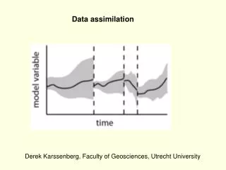
time Forecasting: data assimilation Adjust parameters p, inputs i, and state variables z Compare with state variables z Current and future observations Forecast with calibrated model
Forecasting: data assimilation Time steps with observations
Direct insertion of observations • Replace model state variables with observed variables • Probabilistic techniques using Bayes’ equation • Adjust model state variables • Adjustment is related to uncertainty in model state variables relative to the uncertainty in observations Data assimilation techniques
S: sample space, all possible outcomes (e.g., persons in a test) A: event (e.g., ill person) Ac: complement of A (e.g., person not ill) Note that P(Ac) = 1 - P(A) Understanding Bayes’ equation: Venn diagrams Ac A S
S: sample space, all possible outcomes (e.g., persons in a test) B: event (e.g., person tested positive) Bc: complement of A (e.g., person not tested positive) Understanding Bayes’ equation: Venn diagrams Bc B S
A B: intersection, e.g. persons that are ill and are tested positive Understanding Bayes’ equation: Venn diagrams A B S
P(A|B): conditional probability, the probability of A given that B occurs (e.g. the probability that the person is ill given it is tested positive) Understanding Bayes’ equation: Venn diagrams P(A|B)
Understanding Bayes’ equation: Venn diagrams P(A B) P(B) S
(Ensemble) Kalman filters • Adjust model state by changing state variables of model realizations • Particle filters • Adjust model state by duplicating (cloning) model realizations Data assimilation techniques that use Bayes’ equation
Probabilistic data assimilation for each t set of stochastic variables Solve by using Monte Carlo simulation: n realizations of variables representing state of the model
Apply Bayes’ equation at observation time steps Prior: PDF of observations Prior: PDF model Prior: PDF of observations given the model Posterior: probability distribution function (PDF) of model given the observations
Step 1: Apply Bayes’ equation to realizations of the model Results in a ‘weight’ assigned to each realization Step 2: Clone each realization a number of times proportional to the weight of the realization Apply Bayes’ equation at observation times
text Title Step 2 Step 1
Step 1: Apply Bayes’ equation to each realization (particle) i Prior: PDF of observations Prior: PDF of model realization i Prior: PDF of observations given the model realization i Posterior: probability distribution function (PDF) of realization i given the observations
Proportionality proportional Same for all realizations i
model state observations Calculating weights Measurement error variance of observations
Combine, resulting in ‘weights’ for each realization (particle) proportional
Copy the realizations a number of times proportional to Step 2: resampling Title text Step 2 Step 1
Catchment model: snowfall, melt, discharge • Catchment in Alpes, one winter, time step 1 day • Simplified model for illustrative purposes only • Stochastic inputs: temperature lapse rate, precipitation • Filter data: snow thickness fields
Snow case study • Catchment in Alpes, one winter, time step 1 day • T(s,t) = tarea(t)·L·h(s) for each t T(s,t) temperature field, each timestep tarea(t) average temperature of study area (measured) L lapse rate, random variable h(s) elevation field (DEM)
Snow case study P(t) = parea(t) + Z(t) P(t) precipitation field parea(t) average precipitation of study area (measured) Z(t) random variable with zero mean • Snowmelt linear function of temperature • Filter data: snow thickness fields at day 61, 90, 140
Demo aguila
text Title
text Title
t = 61 t = 90 t = 140 Resampling particles
Visualisations: 1. Realizations Derek Karssenberg et al, Utrecht University, NL, http://pcraster.geo.uu.nl
Visualisations: 2. Statistics calculated over realizations Derek Karssenberg et al, Utrecht University, NL, http://pcraster.geo.uu.nl
Number of Monte Carlo samples per snow cover Interval Probability density Cumulative probability density 0.1
Comparison of Techniques Monte Carlo Particle Filter Ens. Kalman Filter Demo aguila

