Data Assimilation
Data Assimilation. Tristan Quaife, Philip Lewis. What is Data Assimilation?. A working definition: The set techniques the combine data with some underlying process model to provide optimal estimates of the true state and/or parameters of that model. What is Data Assimilation?.


Data Assimilation
E N D
Presentation Transcript
Data Assimilation Tristan Quaife, Philip Lewis
What is Data Assimilation? • A working definition: The set techniques the combine data with some underlying process model to provide optimal estimates of the true state and/or parameters of that model.
What is Data Assimilation? • It is not just model inversion. • But could be seen as a process constraint on inversion (e.g. a temporal constraint)
e.g. Use EO data to constrain estimates of terrestrial C fluxes • Terrestrial EO data: no direct constraint on C fluxes • Combine with model
Data Assimilation is Bayesian • Bayes’ theorem:
What does DA aim to do? • Use all available information about • The underlying model • The observations • The observation operator • Including estimates of uncertainty and the current state of the system • To provide a best estimate of the true state of the system with quantified uncertainty
Kalman Filter DA: MODIS LAI product Data assimilation into DALEC ecological model
Lower-level product DA • Ensure consistency between model and observations • Assimilate low-level products (surface reflectance) • Uncertainty better quantified • Need to build observation operator relating model state (e.g. LAI) to reflectance • Example of Oregon (MODIS DA) • Quaife et al. 2008, RSE
Modelled vs. observed reflectance Red NIR Note BRF shape in red: can’t simulate with 1-D canopy (GORT here)
NEP results No assimilation Assimilating MODIS (red/NIR) DALEC model calibrated from flux measurements at tower site 1
Flux Tower 4.5 km 15 65 gC/m2/year Mean NEP for 2000-2002 Spatial average = 50.9 Std. dev. = 9.7 (gC/m2/year)
NEP – Site2 (intermediate) parameters, with/without DA Model running at Site 2, Oregon Site 1 model EO-calibrated at site 2NEP observations from Site 2 Shows ability to spatialise
Data assimilation • Low-level DA can be effective • ‘easier’ data uncertainties • Can be applied to multiple observation types • Requires Observation operator(s) • RT models • Requires other uncertainties • Ecosystem Model • Driver (climate) • Observation operator
Specific issues in land EOLDAS • No spatial transfer of information • Require full spatial coverage • Atmosphere dealt with by an instantaneous retrieval (i.e. no transport model) • All state vector members influence observations • We are not interested in other variables!
Nominal classification of DA • Sequential • Smoothers • Variational
Sequential methods • Kalman Filter • Variants - EKF • Ensemble Kalman Filter • Variants – Unscented EnKF • Particle filters • Lots of different types • true MCMC technique
The Kalman filter • Propagation step: • x = Mx- • P = MP-MT + Q • Analysis step: • x* = x + K( y – Hx ) • K = PHT( HPHT+R )-1 Model Covariancematrix Stochastic forcing Kalman gain Observation covariance matrix Observation operator State vector Observation vector
The Kalman Filter • Linear process model • Linear observation operator • Assumes normally distributed errors
The Extended Kalman filter • Propagation step: • x = m(x-) • P = M'P-M'T + Q • Analysis step: • x* = x + K( y – h(x) ) • K = PH'T( H'PH'T+R )-1 Jacobian matrix Jacobian matrix
The Extended Kalman Filter • Linear process model • Linear observation operator • Assumes normally distributed errors • Problem with divergence
The Ensemble Kalman filter • Propagation step: • X = m(X-) + Q • no explicit error propagation • Analysis step: • X* = X + K( D – HX ) • K = PHT( HPHT+R )-1 State vector ensemble Perturbed observations
Xa = h(X) X The Ensemble Kalman Filter • P estimated from X • Non linear observations using augmentation:
The Ensemble Kalman Filter No assimilation Assimilating MODIS surface reflectance bands 1 and 2
The Ensemble Kalman Filter • Avoids use of Jacobian matrices • Assumes normally distributed errors • Some degree of relaxation of this assumption • Augmentation assumes local linearisation
Particle Filters • Propagation step: • X = m(X-) + Q • Analysis step: • e.g. Metropolis-Hastings
Particle Filters No available observations
Particle Filters • Fully Bayesian • No underlying assumptions about distributions • Theoretically the most appealing choice of sequential technique, but… • Our analysis show little difference with EnKF • Potentially requires larger ensemble • But comparing 1:1 is faster than EnKF
Sequential techniques • General considerations: • Designed for real time systems • Only consider historical observations • Only assimilates observations in single time step • Can lead to artificial high frequency components
Smoothers • Extension of sequential techniques • All observations effect every time step • Analogous to weighting on observations • [ smoothing-convolution / regularisation ] • Difficult to apply in rapid change areas
Smoothers - regularisation x = (HTR-1H + λ2BTB)-1HTR-1y B is the required constraint. It imposes: Constraint matrix Lagrange multiplier Bf = 0 and the scalar λ is a weighting on the constraint.
Regularisation Quaife and Lewis (2010) Temporal constraints on linear BRDF model parameters. IEEE TGRS, in press.
Regularisation • Lots of literature on the selection of λ • Cross validation etc • Permits insight into the form of Q
Variational techniques • Expressed as a cost function • Uses numerical minimisation • Gradient descent requires differential • Traditionally used for initial conditions • But parameters may also be adjusted
Background Observations 3DVAR • J(x) = ( x-x- ) P-1 ( x-x- )T + • ( y-h(x) ) R-1 ( y-h(x) )T
3DVAR • No temporal propagation of state vector • OK for zero order approximations • Unable to deal with phenology
J(x) = ( x-x- ) P-1 ( x-x- )T + ( y-h(xi) ) R-1 ( y-h(xi) )T Σi Time varying state vector 4DVAR
Variational techniques • Parameters constant over time window • Non smooth transitions • Assumes normal error distribution • Size of time window? • For zero-order case 3DVAR = 4DVAR • 4DVAR for use with phenology model • Absence of Q - propagation of P?
Building an EOLDAS • Lewis et al. (RSE submitted) • Sentinel-2
Assimilation Assume model Uncertainty known
EOLDAS • Base level noise
EOLDAS • Cross validation
EOLDAS • Double noise
Conclusions - technique • DA is optimal way to combine observations and model • Range of options available for DA • Sequential • Smoothers • Variational • Require understanding of relative uncertainties of model and observations • Require way of linking observations and model state • Observation operator (e.g. RT)