Download
1 / 81
900 likes | 1.34k Vues
Mathematical modeling, problem inversion and design of chemical and biological systems. Doctoral Thesis Defense Kedar Kulkarni Date: 10/04/2007 Advisor: Prof. Andreas A. Linninger Thesis committee: Prof. Royston, Prof. Yang Dai, Prof. Hui Lu and Prof. Ali Cinar (IIT)

E N D
Mathematical modeling, problem inversion and design of chemical and biological systems Doctoral Thesis Defense Kedar Kulkarni Date: 10/04/2007 Advisor: Prof. Andreas A. Linninger Thesis committee: Prof. Royston, Prof. Yang Dai, Prof. Hui Lu and Prof. Ali Cinar (IIT) Laboratory for Product and Process Design, Department of Bioengineering, University of Illinois, Chicago, IL 60607, U.S.A.
Motivation: Why Inversion? Data available: Chemical Reactor: (at specific locations) Characteristics:- Partial information available- The system cannot be studied as a whole To determine: Reaction: • Kinetic constants: • Rate of the reaction (k1) • Other constants • Thermal constants: • Thermal conductivity (k) • Porosity (ε) • Diffusivity (D) Microbial growth: Heat transfer: What are the values of k1, μmax, Ks and S0 ?
Brain Tissue Blood Circulation System [18F] Methyl F-DOPA [18F] Methyl F-DOPA Methylation Methylation INJECTION [18F]FDA [18F]FDOPA [18F]FDOPA NH 2 | CH – C – CO H OH 2 2 | CH 3 OH Motivation: Why Inversion? Data available: Drug distribution in the human brain : Characteristics:- Partial information available- Biological system cannot be decomposed into parts To determine: • Kinetic constants: • Metabolic rates of the reaction • Porosity (ε) • Diffusivity (D)
Distributed system data Distributed system data Least squares data-fitting Transport and Kinetic Inversion (TKIP) Black box parameters Physical properties BLACK BOX MODELS 1st PRINCIPLES DISTRIBUTED MODELS HIGH KNOWLEDGE ABOUT THE SYSTEM Filtering/ Data reconciliation LOW KNOWLEDGE ABOUT THE SYSTEM How is Problem Inversion different from least squares data fitting? Model identification: 1st principles models vs. black box models No need for filtering/ data reconciliation for 1st principles model inversion!
Over-design to handle uncertainty Arbitrary overdesign D Feasible operation? Model Optimize D Quantify uncertainty using confidence intervals Guarantee feasible operation Optimize Model Design for nominal condition L Motivation: Why consider design under uncertainty ? Classical process design:MODEL:- Make steady state model of the process- Given design (d) DATA FITTING:Nominal parameter values obtained by least squares optimizationDESIGN FLEXIBILITYEmpirical over-design to accommodate uncertainty
Outline: Problem inversion - Mathematical problem formulation- Previous studies in Inversion- Shortcomings of previous methods- Transport and Kinetic Inversion (Proposed methodology)- Finite volume discretization- Trust region methodsParametric uncertainty- Covariance matrix- Confidence intervalsRisk analysis- Design performance evaluation under uncertainty- Various approaches to quantify design flexibility- Shortcomings of previous methodsCase studies- Case study I – Plutonium storage- Case study II – Discovery of kinetic properties of F-dopa in the human brain- Case study III – Multi-scale analysis and design of a catalytic pellet reactor- Case study IV – Expression flux analysis based inversion of hepatotoxic gene interaction networksConclusions and future research recommendations
Problem inversion-parameter estimation- finite volume discretization- trust region methods Challenges:1) How to handle PDE constraints ?2) Large state variable space3) Efficient algorithmic procedure for inversion
Mathematical Problem Formulation for Inversion Given: Temperature/Concentration Field (from experimental data e.g. MRI) Find: s.t.
Previous studies in inversion: Computational methods • Methods to handle optimization problems with PDE and/or algebraic constraints (Caracotsios and Stewart, 1995)- Least squares optimization problem with PDE constraints (Biegler et al, 2003) Applications • Reaction mechanisms in vapor decomposition processes (Hwang et al, 2005 ) • Inversion in Convective-Diffusive transport problems (Akcelika et al, 2003)- Data assimilation for air-pollution models (Hakami et al, 2003)- Shape optimization (Borgaard and Burns, 1997 )- Reconstruction of tissue-optical property maps (Roy and SevickMuraca, 1999)
Shortcomings of previous methods: 1) They used lumped models Lumped models Distributed models • State variables (e.g. Temperature and concentration) vary spatially and temporally • Did NOT allow the system constants to vary spatially • Scale-up using lumped models is unreliable
Shortcomings of previous methods (cont’d): • 2) No developed theory to quantify coupled transport and reaction • phenomena in distributed systems • 3) No mathematically rigorous method that accounts for the uncertainty • in distributed model parameters and uses confidence interval • information. • 4) There is a lack of efficient algorithmic approaches to quantify the capacity of distributed system design to avoid the violation of constraints (e.g. the safety-critical constraints, the maximum Ph in the bioreactor).
Transport and Kinetic Inversion (Proposed methodology) Initialize parameters, θ Step-1: Discretize PDE constraints • Finite volume methods Step-2: Reduced-space Trust Region Method: (parameters only) • Avoids update of state variables • Robust: Steepest descent • Fast: Quadratic convergence of the Newton • Globally convergent • Robust to ill-conditioning Solvediscretized transport and kinetic constraints (Finite Volume Method). Calculate Newton, ΔθN, and Steepest descent direction, Δθsd Update parameters θnew = θold+ ΔθTR Convergence ? Best fit parameter set, θopt
Finite volume discretization: Transport Model Integrating over a control volume N n e w P E W s y - direction S x- direction Discretization Model (algebraic equations)
True error surface Starting point p1 p2 Trust Region Method: Powell Dogleg Method The dogleg direction combines the Gauss-Newton direction with Steepest descent direction
Parametric uncertainty-Covariance matrix- Individual confidence regions (ICR) - Joint confidence regions (JCR) Challenges:1) How to quantify uncertainty ?2) How to handle parameter correlation ?
Parameter value P(), Probability function = observations - * + Confidence Interval B) Parametric Uncertainty: • How good are the parameter estimates ?- Relax the assumption that parameters are point values- Instead, they are the mean values of a probability distribution function Covariance matrix: The covariance matrix of the parameters contains information regarding the accuracy of their estimates. (Donaldson and Schnabel, 1987)
Obtaining sensitivity information: Transport equations: Implicit differentiation: N is the number of control volumes Linear algebraic system:
2 P(), Probability function Nominal point 2+ 2* 2- 1 1- 1* 1+ = observations 2 2 2 - * + 1 1 Parameter value 1 Confidence Interval ij > 0 ij 0 ij < 0 : Parametric Uncertainty (cont’d): Individual confidence regions (ICR) Joint confidence regions (JCR) Individual confidence regions (ICR) Joint confidence regions (JCR)
Risk analysis-Feasibility test/Flexibility index- Worst case scenario analysis
Design performance evaluation Given the design (d), is its performance feasible even when parameters are varying ? Mathematical representation: Does the rectangle lie wholly inside the feasible region ? Design constraints
Various approaches to quantify design flexibility • Flexibility Analysis (Halemane and Grossmann, 1983, Swaney and Grossmann, 1985): Considers the problem of uncertainty with mathematical rigor - Feasibility Test - Flexibility Index • Optimal Retrofit Design (Pistikopolous and Grossmann, 1988): Optimally redesigning an ‘existing’ process design. • Resilience index (Saboo et al, 1983) • Design reliability (Kubic and Stein, 1988) • Stochastic Flexibility index (Straub and Grossmann, 1983, Pistikopoulos and Mazucchi, 1990) • Convex Hull methods (Ierapetritou et al, 2001)
Feasibility Test * x(d) 0 => feasibility ensured q T * x(d) > 0 => design infeasible for at least one value of q Flexibility Index • F 1 => Flexibility target (F = 1) satisfied • F< 1 => Target (F = 1) not achieved. Fractional F quantifies the maximum tolerable deviation from qN
Approaches to solve flexibility index/ feasibility test problem • Exhaustive enumeration (Swaney and Grossmann, 1985a) - Enumerate all the vertices of the uncertain hyper cube • Implicit vertex enumeration and heuristic vertex search (Swaney and Grossmann, 1985b) - Informed enumeration of vertices of uncertain hyper cube • Active constraint formulation (Grossmann and Floudas, 1987) - Use of KKT conditions to solve a single-level optimization problem by infeasible path methods • Convex Hull methods (Ierapetritou et al, 2001) - Inscription of a convex hull in the feasible region using chosen boundary points • Deterministic global optimization methods – a-BB algorithm (Floudas et al, 2001) - Relaxation of feasible region based on convexification of constraints
Shortcomings of previous approaches: Three important shortcomings of existing methods: • Feasibility test/ flexibility index problems involve non- differentiabilities (e.g. min, max functions) - Gradient based methods not well-suited! (2) Feasibility test/ flexibility index are deterministic global concepts. - A majority of existing gradient based methods evaluate the local optima barring a few exceptions (a-BB, BARON) (3) Not suited for solving (Non) linear infinite programs (NLIP’s) - Cannot handle the infinite space dimensionality in the parameter domain
DOE safety requirements regarding the safe storage of Plutonium dioxide powder for 50 years Temperature increase could leads to an overall pressure increase: could lead to explosion Obtain values of the heat generation (q), the heat transfer coefficient (U) and the thermal conductivity (k) via inversion Select the most adequate model using model-selection metrics Quantify parametric uncertainty through effective use of the covariance information Use flexibility analysis/feasibility test concepts to identify the worst case temperature hotspot in the system Case Study I: Plutonium Storage Background and motivation: Are we safe ?! Objectives:
Experimental setup Radial temperature measurements available 5.7 cm from the bottom of the vessel Actual cylinder (Bielenberg et al, 2004) Schematic
Problem formulation To determine: a) Nuclear heat generation, q, W/m3 b) Effective thermal conductivity, k, J/(K. s.m2) c) Wall heat transfer coefficients, U, W/m.K Math program: s.t. BC’s:
Overall methodology Inversion problem Obtain experimental data • Inversion problem- parameter estimation- finite volume discretization- trust region methodsB) Parametric Uncertainty- Covariance matrix- Confidence intervals (individual and joint)C) Risk analysis- Worst case temperature hotspot using a bi-level optimization problem Select model and estimate parameters by solving inversion problem Parametric Uncertainty Confidence intervals/ Joint confidence regions Risk analysis Feasibility test/ Flexibility index Worst case scenario
A) Inversion problem: 1) Obtain experimental data: Temperature measurements at 6 radial points 5.7 cm from the bottom of the cylinder 2) Solve the math program:
Finite Volume Discretization: Use FVM to render PDE constraints to algebraic equations FVM
3) Select the most adequate model - Which of the following five models describes the data the best ? Models A - E Increasing order of complexity
4) Select the most adequate model (cont’d) Metrics for comparison of models: a) Least Squares Error and b) the F - ratio Sum of squared error between model and expt. data Helps choose the model with the ‘optimal’ degrees of freedom(The largest model is NOT always the best !!) (Froment and Bischoff, 1990) Best fit parameters Model quality Model comparison: Model D is the best using these metrics !
4) Results - Simulation model with the estimated parameters: Model Boundary conditions Optimal Parameters Experimental data and simulated radial temperature-profiles at different pressures at height z = 5.7 cm (12 radial and 10 vertical nodes).
5) Results for confidence bounds using sensitivity information: Individual confidence regions (ICR) Joint confidence regions (JCR) Covariance matrix for q and U: ICR
Results for confidence bounds of two and three parameters: JCR and ICR (2) JCR (3)
(W/m2.K) (W/m3) C) Risk Analysis (Identification of worst case hotspot): Temperature Contours (isotherms) Solution: (a) JCR worst case T – 704 K (b) ICR worst case T – 711 K Locus of the temperature hotpot
Publications: Archival journals: • Kedar Kulkarni, Libin Zhang, Andreas A Linninger, “Model and Parameter uncertainty in Plutonium Storage”, Industrial and Engineering Chemistry Research, 2006 (Accepted with minor revisions). • Libin Zhang, Kedar Kulkarni, MahadevaBharath R. Somayaji, Michalis Xenos and Andreas A Linninger, “Discovery of Transport and Reaction Properties in Distributed Systems”, AIChE Journal, 2006 (Accepted with minor revisions) • Libin Zhang, Andres Malcolm, Kedar Kulkarni, Celia Xue, Andreas A Linninger , “Distributed System Design Under Uncertainty”, Industrial and Engineering Chemistry Research, 2006 (Accepted with minor revisions). Conference papers and presentations: • Kedar Kulkarni, Libin Zhang and Andreas A. Linninger, “Model and Parameter Uncertainty in Plutonium Storage”, AIChE Chicago Section Symposium, Northwestern University, Chicago, IL, USA, April 12, 2006. • Libin Zhang, Kedar Kulkarni, Andres Malcolm, “Modeling Uncertainty Analysis in Distributed Systems”, Design of Integrated Chemical and Biological Systems,AIChE 2005 Annual Meeting, Cincinnati, Ohio, USA, October 30-November 4, 2005. • Libin Zhang, MahadevaBharath R. Somayaji, Michalis Xenos, Kedar Kulkarni, Andreas A. Linninger, “Large Scale Transport and Kinetic Inversion Problem for Drug Delivery into the Human Brain”, “Chemical Engineering at the Cross Roads of Technology”, AIChE April 2005 Symposium, Illinois Institute of Technology, Chicago, IL, USA, April 19 -20, 2005.
Case Study II: Discovery of unknown transport and metabolic/kinetic properties of F-Dopa Problem formulation: s. t. Convection-Diffusion equation Transport of the bulk fluid Concentration field obtained from imaging data Model predicted concentration field of the drug Covariance matrix of the measurements To find:
NH 2 | CH – C – CO H OH 2 2 | CH 3 OH Discovering metabolic properties for F-Dopa Brain Tissue Blood Circulation System [18F] Methyl F-DOPA [18F] Methyl F-DOPA Methylation Methylation INJECTION [18F]FDA [18F]FDOPA [18F]FDOPA L-Dopa Methyl Dopa L-Dopa Dopamine To determine: Blood-tissue clearance K1 Tissue-blood clearance k2 The diffusivities DD , DM s. t. F-dopa clearance Methyl F- dopa clearance
0.09 0.08 0.07 0.06 0.05 0.04 0.03 0.02 0.01 0 Clinical concentration field of F-dopa Unstructured computational grid s. t. Fdopa clearance Methyl - Fdopa clearance Results: Discovering metabolic properties for F-Dopa Putamen Predicted F-Dopa concentration field with optimal parameters ( Gjedde, A. et. al. Neurobiology, 88, 2721-2725, 1991 ) Best-fit Parameters:
Publications: Archival journals: • Libin Zhang, Kedar Kulkarni, MahadevaBharath R. Somayaji, Michalis Xenos and Andreas A Linninger, “Discovery of Transport and Reaction Properties in Distributed Systems”, AIChE Journal, 2006 (Accepted with minor revisions) Conference papers and presentations: • Libin Zhang, MahadevaBharath R. Somayaji, Michalis Xenos, Kedar Kulkarni, Andreas A. Linninger, “Large Scale Transport and Kinetic Inversion Problem for Drug Delivery into the Human Brain”, “Chemical Engineering at the Cross Roads of Technology”, AIChE April 2005 Symposium, Illinois Institute of Technology, Chicago, IL, USA, April 19 -20, 2005. • Kedar Kulkarni, Jeonghwa Moon, Libin Zhang and Andreas Linninger, “Solution Multiplicity of Inversion Problems in Distributed Systems”, Applied Mathematics in Bioengineering, AIChE 2006 Annual Meeting, San Fransisco, California, USA, November 12 – 17, 2006 (Abstract accepted).
Cooling Outlet Multi-scale Model B A Tubular Reactor Cooling inlet Packed Catalyst Pellet Bed Catalyst Pellets Micro Pores of Catalysts Case Study III: Multi-scale analysis and design of the catalytic pellet reactor BULK (MACROSCOPIC) MODEL Mass and energy balances PELLET (MICROSCOPIC) MODEL Coupled mass and energy balance
Problem formulation To determine: a) Bulk diffusivity of species A, DA, m2/s b) Reference reaction constant, kref, 1/s c) Activation energy, E, J/mol Math program: s. t. BC’s:
Overall methodology • Inversion problem- parameter estimation- finite volume discretization- trust region methodsB) Design under uncertainty- Covariance matrix- Confidence intervals (individual and joint)- Cost analysis - Sampling
Optimal Parameters: DA = 0.732 10-4 (m2/s) ; kref= 0.8 10-4 (1/s); E = 5268.62 (J/mol) A) Inversion problem (Results) Concentration profile Temperature profile C T Length of the reactor Length of the reactor
Inversion solution multiplicity Possible reasons: 1) Erroneous datasets 2) Multiple datasets 3) Highly nonlinear coupled pellet PDE’s Different initial guesses gave different solutions!
B) Design under uncertainty Objective: To obtain optimal design and cooling policy by minimizing expected costConstraints: (i) Product quality constraint (ii) Safety constraint Method: Sampling in the individual and joint confidence regions of the uncertain parameters Problem formulation: s. t. Conversion threshold Maximum admissible temperature