ANOVA notes
ANOVA notes. NR 245 Austin Troy Based primarily on material accessed from Garson, G. David 2010. Univariate GLM, ANOVA, and ANCOVA. Statnotes : Topics in Multivariate Analysis. http://faculty.chass.ncsu.edu/garson/PA765/statnote.htm. Central tendency refresher. Mean Median Variance

ANOVA notes
E N D
Presentation Transcript
ANOVA notes NR 245 Austin Troy Based primarily on material accessed from Garson, G. David 2010. Univariate GLM, ANOVA, and ANCOVA. Statnotes: Topics in Multivariate Analysis. http://faculty.chass.ncsu.edu/garson/PA765/statnote.htm
Central tendency refresher • Mean • Median • Variance • Standard Deviation Variance for population For sample
ANOVA • “main effect” vs interactive effects of categorical independent variables (factors) on a continuous/interval dependent • Tests for overall differences in means, not variances • Pairwisecomparisons
Whether difference exists depends on: • Size of differences between group means. • Sample sizes in each group. • Variances of dependent variable by group
Fixed vs. random effects ANOVA • Fixed: data are collected on all categories of independent variables. • Factors with all category values included are "fixed factors." • Random effect ("Model II"), data collected only for a partial sample of categories. • One-way ANOVA: computation of F is the same for fixed and random effects • Mixed effects models with both types
Research design: between groups • Dependent variable is measured for independent groups of sample members, where groups represent different condition, or categories. • Experimental mode: conditions assigned randomly to subjects, or subjects assigned randomly to conditions • Non-experimental mode, conditions are measures of the independent variable for each group.
Full factorial ANOVA • More than one factor: two-way or higher • In this approach, each cell becomes a “group” Source: http://faculty.chass.ncsu.edu/garson/PA765/anova.htm
ANOVA assumptions • Interval data. • nonparametric Kruskal-Wallace • Homogeneity of variances. • Box plots • Multivariate normality.
ANOVA assumption • Adequate sample size. • Random sampling • Equal or similar sample sizes.
Interpretting2+way ANOVA • Profile plots • Color= 2nd factor (e.g. gender) • Parallel lines= lack of interaction effects • Separate lines = different means based on gender • Triangle or X= different groups means based on region • Bottom row: both effects plus interaction Source: http://faculty.chass.ncsu.edu/garson/PA765/anova.htm
F test for comparing group means • For most designs, F is between-groups mean square variance divided by within-groups MSV • If F >1, then there is more variation between groups than within groups, = the grouping variable does make a difference. • Significance of F stat: using df=k-1 (between group; df for numerator) and df=N-k-1 (within group; df for denominator) • Larger the ratio of between-groups variance (signal) to within-groups variance (noise), the less likely that the null hypothesis is true=more variation between groups than within groups
Pairwise comparisons • Assess group differences • The possible number of comparisons is k(k-1)/2. • For two comparisons use standard t test • For more comparisons: • Bonferronitest: like t-test but adjust the significance level by multiplying by the number of comparisons being made. • Tukey’s HSD test: like a t-test, but corrects for experiment-wise error rate; gives conservative results when group sizes are unequal; good with large number of categories.
ANOVA outputs • Example: pain level by analgesic drug group • Rsquare is model of goodness of fit and is often referred to as “partial eta squared” for ANOVA= ratio of the between-groups sum of squares to the total sum of squares • Adjusted R-square adjusts the Rsquare value to penalize for more parameters by using the degrees of freedom in its computation R-adj= 1 - SSE(n-1)/SST(v) • Root MSE gives the standard deviation of the random error • Mean of response gives sample mean
ANOVA outputs • This section gives F test results • DF= degrees of freedom • Sum of Squares C. Total= sum of squared distances of each response from the sample mean; Error is the residual or unexplained SS after fitting the model • Mean square is a sum of squares divided by its associated df • F score is ratio of the Model mean square to the error mean square • Prob>F is p value; observed significance probability of obtaining a greater F-value by chance alone. 0.05 or less considered evidence of a regression effect. • Also get Mean, Std Error (in this case is the root mean square error divided by square root of the number of values used to compute the group mean. and confidence intervals for each group
ANOVA outputs-comparisons • Top: LSD Threshold matrix: absolute difference in the means minus the LSD, which is the minimum difference that would be significant. Pairs with a positive value are significantly different. The q statistic is a scaling variable • Next table: significant differences based on the letters that apply to them (A, B) • Final table gives all pairwise comparisons. Gives differences, confidence intervals and p value. Those with significant differences are starred • Also gives diamond and circle plots. If two circles overlap significantly, those groups are not different
Box plot Outliers are either 3×inter-quartile range (the width of the box in the box-and-whisker plot) or more above the third quartile or 3×IQR or more below the first quartile