CEM in action
750 likes | 958 Vues
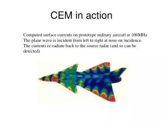
CEM in action. Computed surface currents on prototype military aircraft at 100MHz The plane wave is incident from left to right at nose on incidence. The currents re-radiate back to the source radar (and so can be detected). 83 Camaro at 1 GHz.

CEM in action
E N D
Presentation Transcript
CEM in action Computed surface currents on prototype military aircraft at 100MHz The plane wave is incident from left to right at nose on incidence. The currents re-radiate back to the source radar (and so can be detected)
83 Camaro at 1 GHz • Irradiation of a 83 Camaro at 1 GHz by a Hertzian dipole.
Simulation Measurement > 2,000,000 unknowns Inlet Scattering
Microstrip Antenna Array Radiation patterns Current distribution
EMP Microwave pulse penetrating a missile radome containing a horn antenna. Wave is from right to left at 15° from boresight.
20 cm 10 cm 5 cm 1 cm 17.5 cm Voltages on the varistors 0.5 cm 6 cm 4.5 cm 25 cm 25 cm Voltage (kV) 15 cm 500 1 cm 500 y z y x Broadband Analysis of Wave Interactions with Nonlinear Electronic Circuitry EM solvers permit analysis of wave broadband EMC/EMI phenomena, and the assessment of electronic upset and terrorism scenarios
AZ Memory Matrix-fill LUD One-RHS (GB) (days) (years) (hrs) 5 0.1 9 32,000 600.0 200 4 32,000 600.0 500 FIES LUD CG Scattering at 3 GHz from Full Fighter Plane (fast solvers) Bistatic RCS of VFY218 at 3 GHz 8 processors of SGI Origin 2000 # of Unknowns N = 2 millions
computational electromagnetics rigorous methods High frequency DE current based IE VM field based TD FD TD FD PO/PTD FDTD TLM FEM MoM GO/GTD Computational Electromagnetics
Computational Electromagnetics Electromagnetic problems are mostly described by three methods: Differential Equations (DE) Finite difference (FD, FDTD) Integral Equations (IE) Method of Moments (MoM) Minimization of a functional (VM) Finite Element (FEM) Theoretical effort less more Computational effort more less
Fields • Fields: A space (and time) varying quantity • Static field: space varying only • Time varying field: space and time varying • Scalar field: Magnitude varies in space (and time) • Vector field: Magnitude & direction varies in space (and time) Moving Fields…... Electromagnetic waves
Real, time harmonic scalar Complex Number (Phasor) Phasor Transform P Time Harmonic Fields • Fields that vary periodically (sinusoidally) with time Time Harmonic Scalar Fields
Maxwell’s Equations in Differential Form Faraday’s Law Ampere’s Law Gauss’s Law Gauss’s Magnetic Law
Faraday’s Law C S
Gauss’s Magnetic Law (no magnetic charges!) “all the flow of B entering the volume V must leave the volume”
CONSTITUTIVE RELATIONS e=er eo=permittivity (F/m) eo=8.854 x 10⁻¹² (F/m) m=mr mo=permeability (H/m) mo=4p x 10-7 (H/m) s=conductivity (S/m)
POWER and ENERGY Stored magnetic power (W) Supplied power (W) What is this term? Dissipated power (W) Stored electric power (W)
POWER and ENERGY Stored magnetic power (W) Supplied power (W) What is this term? Dissipated power (W) Stored electric power (W) Ps = power exiting the volume through radiation W/m2 Poynting vector
TIME HARMONIC EM FIELDS Assume all sources have a sinusoidal time dependence and all materials properties are linear. Since Maxwell’s equations are linear all electric and magnetic fields must also have the same sinusoidal time dependence. They can be written for the electric field as: Euler’s Formula is a complex function of space (phasor) called the time-harmonic electric field. All field values and sources can be represented by their time-harmonic form.
PROPERTIES OF TIME HARMONIC FIELDS Time derivative: Time integration:
TIME HARMONIC MAXWELL’S EQUATIONS Employing the derivative property results in the following set of equations:
PEC Boundary Conditions TIME HARMONIC EM FIELDSBOUNDARY CONDITIONS AND CONSTITUTIVE PROPERTIES The constitutive properties and boundary conditions are very similar for the time harmonic form: General Boundary Conditions Constitutive Properties
s2,e2,m2 s1,e1,m1 s1>> s2 TIME HARMONIC EM FIELDSIMPEDANCE BOUNDARY CONDITIONS If one of the material at an interface is a good conductor but of finite conductivity it is useful to define an impedance boundary condition:
POWER and ENERGY: TIME HARMONIC Time average magneticenergy (J) Supplied complex power (W) Time average electric energy (J) Dissipated real power (W) Time average exiting power
CONTINUITY OF CURRENT LAW vector identity time harmonic
SUMMARY Time Domain Frequency Domain
Wave Equation Time Dependent Homogenous Wave Equation (E-Field) Vector Identity
Source Free Wave Equation Source-Free Time Dependent Homogenous Wave Equation (E-Field) Source-Free Lossless Time Dependent Homogenous Wave Equation (E-Field) Lossless
Source Free Wave Equation Source-Free Time Dependent Homogenous Wave Equation (H-Field) Source Free and Lossless
Source Free Source Free Wave Equation: Time Harmonic Time Domain Frequency Domain Lossless Lossless “Helmholtz Equation”
MOST POPULAR COMPUTATIONALELECTROMAGNETICS ALGORITHMS • FINITE DIFFERENCE (FD) METHODS • Example: Finite difference time domain (FDTD) • INTEGRAL EQUATION METHODS (IE) • Example: Method of Moments (MoM) • VARIATIONAL METHODS • Example: Finite element method (FEM)
Conventional Calculus The operation of diff. of a function is a well-defined procedure The operations highly depend on the form of the function involved Many different types of rules are needed for different functions For some complex function it can be very difficult to find closed form solutions Numerical differentiation Is a technique for approximating the derivative of functions by employing only arithmetic operations (e.g., addition, subtraction, multiplication, and division) Commonly known as “finite differences” Introduction to differentiation
y f(x) xi x f(xi) Taylor Series Problem: For a smooth function f(x), Given: Values of f(xi) and its derivatives at xi Find out: Value of f(x) in terms of f(xi), f(xi), f(xi), ….
Taylor’s Theorem If the function f and its n+1 derivatives are continuous on an interval containing xiand x, then the value of the function f at x is given by
Finite Difference Approximationsof the First Derivative using the Taylor Series (forward difference) Assume we can expand a function f(x) into a Taylor Series about the point xi+1 y f(x) h xi xi+1 x f(xi) f(xi+1) h
Finite Difference Approximationsof the First Derivative using the Taylor Series (forward difference) Assume we can expand a function f(x) into a Taylor Series about the point xi+1 Ignore all of these terms
Finite Difference Approximationsof the First Derivative using the Taylor Series (forward difference) y f(x) h xi xi+1 x f(xi) f(xi+1)
Finite Difference Approximationsof the First Derivative using the forward difference: What is the error? The first term we ignored is of power h1. This is defined as first order accurate. First forward difference
Finite Difference Approximationsof the First Derivative using the Taylor Series (backward difference) Assume we can expand a function f(x) into a Taylor Series about the point xi-1 y f(x) h xi-1 xi x f(xi-1) f(xi) -h
Finite Difference Approximationsof the First Derivative using the Taylor Series (backward difference) Ignore all of these terms First backward difference
Finite Difference Approximationsof the First Derivative using the Taylor Series (backward difference) y f(x) h xi-1 xi x f(xi-1) f(xi)