Poynting’s theorem
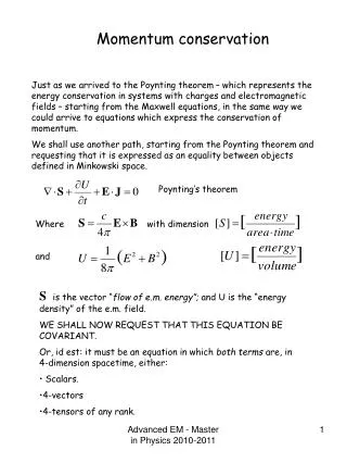
Momentum conservation. Just as we arrived to the Poynting theorem – which represents the energy conservation in systems with charges and electromagnetic fields – starting from the Maxwell equations, in the same way we could arrive to equations which express the conservation of momentum.

Poynting’s theorem
E N D
Presentation Transcript
Momentum conservation Just as we arrived to the Poynting theorem – which represents the energy conservation in systems with charges and electromagnetic fields – starting from the Maxwell equations, in the same way we could arrive to equations which express the conservation of momentum. We shall use another path, starting from the Poynting theorem and requesting that it is expressed as an equality between objects defined in Minkowski space. Poynting’s theorem Where and with dimension • S is the vector “flow of e.m. energy”; and U is the “energy density” of the e.m. field. • WE SHALL NOW REQUEST THAT THIS EQUATION BE COVARIANT. • Or, id est: it must be an equation in which both terms are, in 4-dimension spacetime, either: • Scalars. • 4-vectors • 4-tensors of any rank. Advanced EM - Master in Physics 2010-2011
So, let us examine the Poynting theorem with Professor Lorentz’s eye. • Two remarks: • The first two terms are a divergence and a derivative over • time: they could (should!) together belong to a that has been written with the “c” constant for generality. • 2. The third termE·J is a three-dimensional scalar product made with the components of vector J, which are the “space” components of the 4_current [-cρ,-J], and with the components of the column 0 of the FIELD TENSOR: CONCLUSION: The extension to spacetime of the Poynting theorem is an equality between two 4-vectors! Because the original equation of the Poynting’s theorem must be the equality between the two time_components of two 4-vectors! Advanced EM - Master in Physics 2010-2011
The term, will therefore have to be the product of ∂μ with an object that can only be the row “time” of a 4-TENSOR of rank 2. And the equation of Poynting’s theorem becomes: In these equation the terms of the first column are well known, since they are: The components of the tensor Tμνare therefore products of the components of the fields. Since we have two different expressions for the fields, there are 4 possibilities for the tensor Tμν . It turns out that the correct form for Tμ0is: Advanced EM - Master in Physics 2010-2011
This equation valid for the column zero (time_) of the tensor Tμν is therefore valid for all columns! And we eventually have: Advanced EM - Master in Physics 2010-2011
Requesting that the equation of the Poynting’s theorem be covariant means requesting that – once ascertained that in its original form it is the condition of equality of the “time” components of two 4-vectors – that equality holds also for the three “space” components of the two 4-vectors. The Poynting’s theorem becomes this equality between all 4 components of the two 4-vectors: From this generalization we obtain three scalar equations, which we must understand. Of course, since the fourth equation, from which we derived the last three, is the conservation of energy: it is simply obvious to expect that the other three express the conservation of linear momentum. We have however now three scalar equations, which we can write down because we know all their terms, and we must interpret them, independently from our assumptions. Before writing down the three equations explicitly we take a second, better look at the tensor Tμν: beside the first row and column, whose meaning we know already, there are another nine elements which form a submatrix 3*3 which, on a better look, reveals itself as an old “friend”: the Maxwell stress tensor (with opposite sign). We can therefore use this shorthand for the Tμν tensor: Advanced EM - Master in Physics 2010-2011
The three scalar equations between the space-components of the two 4-vectors are: In this equation the right-hand term is the Lorentz force which acts on a distribution of charge and current. Given the equation of Newtonian mechanics F=dP/dt we can say that the second term of this equation is the variation in time dP/dtof the charge system. The equation concerns then the change with time of linear momenta of various players. Beside the charges and their currents the only other player is the field itself. We can therefore assume that the time derivative of S/c² will also be the variation with time of the density of linear momentum , but that of the field! We therefore have that, if we integrate over the charge contained in a given finite volume, the following equation holds: Where Fi is the component along axis “i” of the total force applied by the field over the volume V. Advanced EM - Master in Physics 2010-2011
There is something to say about the previous formulas. In the first place, note that the components of the Maxwell stress tensor (3·3 elements) have opposite sign of the related elements of Tμν. Then, in a tensor the elements of a row or of a column are transformed – for a change of reference axes – as components of a vector. This is the reason why we have applied – in the 4th passage, the Gauss theorem, which applies to vectors. The final equation we have come up with, and which represents the extension of Poynting’s theorem, i.e. the momentum conservation, is: where the term on the right side is the total “force” exerted by the fields on the electrical content of the volume – charges and fields. Rather than a plain force, it represents a “Momentum flow” through the surface enclosing the volume. And,… it is the momentum carried by the fields, since in the formulae of the components of Tμνonly the fields enter. When we discussed the stress tensor in 3 dimensions we only studied the force exerted by the fields on the charges , and came up with the Maxwell’s stress tensor. Now we have extended the study to the whole balance of momentum and energy, and have come up with a new vector g that represents the momentum distribution of the fields. is the momentum density of the fields. Advanced EM - Master in Physics 2010-2011
We already know the fields of a point charge in uniform motion (at relativistic speed). And also know that the Poynting’s vector in that case is directed along the direction of the charge’s movement, is very strong in the plane orthogonal to the direction of motion and including the charge. Now we know that this very Poynting’s vector is also proportional to something that turns out to be is momentum of the field, which adds up to the mechanical momentum of the charge. We started at the beginning of this course by finding that there is an energy associated with fields, and also that this energy can belong to the fields themselves once they have been created, and not to their interaction with charges. Now, with the request that the equations be valid in 4-dimensional spacetime (covariance) we find that fields also carry momentum. There is another subject we need to deal with before leaving the subject of electromagnetism and relativity. We know that charged particles in acceleration radiate e.m. fields. And we know that these fields carry their own electromagnetic energy. But… how much of the accelerated particle energy is radiated out? That can be calculated. But, the radiation fields (Lienard and Wiechert), those who actually take their own energy and carry it away, have a dependence on the acceleration a and on the scalar product a·β, so the emitted power depends on the angle between acceleration and velocity . We have been able to compute the radiated power by an accelerated charge in a frame in which the charge is at rest: the Larmor formula. We would like to extend the calculation to charges in motion, and see what happens at relativistic speeds. That is not too difficult. Now we know how to handle phenomena seen in different IRFs, if we know the values of some quantities in one IRF we “easily” compute in other frames, like those in which charges have any velocity. Advanced EM - Master in Physics 2010-2011
Relativistic extension of the Larmor formula. To find the e.m. power radiated by a charge in arbitrary motion, i.e. with arbitrary values of the two vectorsa and β we need to transform the IRF into the IRF’ in which the charge is at rest, calculate the acceleration a’there and compute the emitted power there with the Larmor formula: Where U is the energy radiated and Wthe power. We know the motion of the charge in IRF, and we need to apply a Lorentz transformation to the system IRF’ where it is at rest, and compute a’as a function of a. We can then compute W’ with the Larmor formula. The next step is simple, because it turns out that W = W’ i.e. dU/dt is a Lorentz invariant. At this point we only need to substitute for a’ its value as a function of a and β. We make now use of the derivation of the 4-acceleration in lesson 16. The formula for the 4-acceleration as a function of the 3-dimensional v and a is: Advanced EM - Master in Physics 2010-2011
Lorentz transformation where Λis the matrix of the Lorentz transformation. Let us choose IRF and IRF’ with their x-axes directed along the direction of relative motion: v =(v,0,0) v’ = (0,0,0) The charge 4-acceleration (the thing we want to pass from one IRF to the other via the Lorentz transformation) is, in the two IRFs: where β=v/c. Remember, our goal is to express a’as a function ofa. This connection is achieved by writing down the Lorentz transformation relating . We now write down the Lorentz transformation of all 4 components of the 4-acceleration. These 4 equations provide the values of a’i as a function of ai : Advanced EM - Master in Physics 2010-2011
Velocity and acceleration PARALLEL: Velocity and acceleration ORTHOGONAL: This formula shows that the x_coordinate is treated differently from the other two. The reason is obvious: the charge’s velocity is directed along the x-axis. As a consequence, the radiation will have different power for accelerations parallel to the velocity or orthogonal to it. That is because, as we said, W = W’ i.e. dU/dt is a Lorentz invariant. Therefore: which is the relativistic generalization of the Larmor formula. It is interesting to look at the two cases separately: Advanced EM - Master in Physics 2010-2011
Comparing this result with the original Larmor formula we see that the correction for relativistic velocities becomes very large: • This increase of the emitted radiation for relativistic particles is mostly due to the fact that, when β≈1 the accelerations can be very small even for large variations in momentum. • Another remark: the two cases treated above, of velocity and acceleration parallel or orthogonal to each other are fairly common in nature: • the first (parallel) is the case of head-on collision of particles, and has taken the name of bremsstrahlung. • The second case (orthogonal) is the typical case of motion of charged particles in magnetic fields, and is called synchrotron radiation (the magnetic force is always perpendicular to the charge’s velocity). Advanced EM - Master in Physics 2010-2011