ECONOMIC GROWTH
ECONOMIC GROWTH. Lviv, September 2012. Growth in Finland. The Sources of Economic Growth. Production function Y = AF ( K , N ) Decompose into growth rate form: the growth accounting equation D Y / Y = D A / A + a K D K / K + a N D N / N

ECONOMIC GROWTH
E N D
Presentation Transcript
ECONOMIC GROWTH Lviv, September 2012
The Sources of Economic Growth • Production function Y = AF(K, N) • Decompose into growth rate form: the growth accounting equation DY/Y =DA/A + aKDK/K + aNDN/N • The a terms are the elasticities of output with respect to the inputs (capital and labor)
The Sources of Economic Growth • Interpretation • A rise of 10% in A raises output by 10% • A rise of 10% in K raises output by aK times 10% • A rise of 10% in N raises output by aN times 10% • Both aK and aN are less than 1 due to diminishing marginal productivity
The Sources of Economic Growth • Growth accounting • Four steps in breaking output growth into its causes (productivity growth, capital input growth, labor input growth) • Get data on DY/Y, DK/K, and DN/N, adjusting for quality changes • Estimate aK and aN from historical data • Calculate the contributions of K and N as aKDK/K and aNDN/N, respectively • Calculate productivity growth as the residual: DA/A=DY/Y – aKDK/K – aNDN/N
The Sources of Economic Growth • Growth accounting and the productivity slowdown • Denison’s results for 1929–1982 • Entire period output growth 2.92%; due to labor 1.34%; due to capital 0.56%; due to productivity 1.02% • Pre-1948 capital growth was much slower than post-1948 • Post-1973 labor growth slightly slower than pre-1973
Sources of Economic Growth in the United States (Denison) (Percent per Year)
Productivity Labor TFP Growth rate Productivity of K/N Labor productivity growth may exceed TFP growth because of faster growth of capital relative to growth of labor
Technological Progress in the Solow Model • A new variable: E = labor efficiency • Assume: Technological progress is labor-augmenting: it increases labor efficiency at the exogenous rate g = ∆E/E: • We now write the production function as: Y = F(K,L*E) where L*E is the number of effective workers. • Increases in efficiency will have the same effect on output as increases in the labor force.
The Solow Model • Basic assumptions and variables • Population and work force grow at same rate n • Economy is closed and for now there is no govt. (G= 0) Ct=Yt – It • Rewrite everything in per-worker terms: (kt is also called the capital-labor ratio) • Therefore, saving and investment per effective worker is: sy=sf(k)
The Solow Model • The per-worker production function yt=f(kt) • Assume no productivity growth for now (we will add it later) • Plot of per-worker production function • Same shape as aggregate production function
The Solow Model • Steady states • Steady state: yt, ct, and kt are constant over time • Gross investment must • Replace worn out capital, δKt • Expand so the capital stock grows as the economy grows, nKt • Provide capital for the new “effective” workers created by technological progress, It= (δ+n+g)Kt • If so, then ( +n +g)k = break-even investment: the amount of investment necessary to keep k constant.
The Solow Model • Ct=Yt – It=Yt – (δ+n+g)Kt • In per-worker terms, in steady state c=f(k) - (δ+n+g)kt • Plot of c, f(k), and (δ+n+g)kt
The relationship of consumption per worker to the capital–labor ratio in the steady state
The Solow Model • Increasing k will increase c up to a point • This is kG in the figure, the Golden Rule capital-labor ratio • For k beyond this point, c will decline • But we assume henceforth that k is less than kG, so c always rises as k rises
The Solow Model • Reaching the steady state • Suppose saving is proportional to current income: St=sYt, where s is the saving rate, which is between 0 and 1 • Equating saving to investment gives sYt= (n+d + g)Kt
The Solow Model • Putting this in per-worker terms gives sf(k) = (n+ δ + g)k • Plot of sf(k) and (n+ δ + g)k
The steady state • The only possible steady-state capital-labor ratio is k* • Output at that point is y* = f(k*); consumption is c* = f(k*) – (n + d + g)k* • If k begins at some level other than k*, it will move toward k* • For k below k*, saving > the amount of investment needed to keep k constant, so k rises • For k above k*, saving < the amount of investment needed to keep k constant, so k falls
Long-run growth • To summarize: With no productivity growth, the economy reaches a steady state, with constant capital-labor ratio, output per worker, and consumption per worker. • Therefore, the fundamental determinants of long-run living standards are: • The saving rate • Population growth • Productivity growth
The fundamental determinants of long-run living standards: the saving rate • Higher saving rate means higher capital-labor ratio, higher output per worker, and higher consumption per worker
The fundamental determinants of long-run living standards: population growth • Higher population growth means a lower capital-labor ratio, lower output per worker, and lower consumption per worker
Fundamental Determinants of Long-run Living Standards: Productivity Growth • In equilibrium, productivity improvement increases the capital-labor ratio, output per worker, and consumption per worker: Productivity improvement directly improves the amount that can be produced at any capital-labor ratio and the increase in output per worker increases the supply of saving, causing the long-run capital-labor ratio to rise
Growth Empirics: Balanced growth • Solow model’s steady state exhibits balanced growth - many variables grow at the same rate. • Solow model predicts Y/L and K/L grow at the same rate (g), so K/Y should be constant. This is true in the real world. • Solow model predicts real wage grows at same rate as Y/L, while real rental price is constant. Also true in the real world.
Growth Empirics: Convergence • Solow model predicts that, other things equal, “poor” countries (with lower Y/L and K/L) should grow faster than “rich” ones. • If true, then the income gap between rich & poor countries would shrink over time, causing living standards to “converge.” • This does not always occur because “other things” aren’t equal. • In samples of countries with similar savings & pop. growth rates, income gaps shrink about 2% per year. • In larger samples, after controlling for differences in saving, pop. growth, and human capital, incomes converge about 2% per year.
Factor Accumulation vs. Production Efficiency • Differences in income per capita among countries can be due to differences in: 1. capital – physical or human – per worker 2. the efficiency of production (the height of the production function) • Empirical studies find that: • Both factors are important. • The two factors are correlated: countries with higher physical or human capital per worker also tend to have higher production efficiency.
Endogenous Growth Theory • Endogenous growth theory—explaining the sources of productivity growth • Aggregate production function Y = AK • Constant Marginlal Product of Kapital • Human capital • Knowledge, skills, and training of individuals • Human capital tends to increase in the same proportion as physical capital • Research and development programs • Increases in capital and output generate increased technical knowledge, which offsets decline in MPK from having more capital
Endogenous Growth Theory • Implications of endogenous growth • Suppose saving is a constant fraction of output: S = sAK • Since investment = net investment + depreciation, I =DK + dK • Setting investment equal to saving implies: DK + dK = sAK • Rearrange: DK/K = sA – d • Since output is proportional to capital, DY/Y = DK/K, so DY/Y = sA – d • Thus the saving rate affects the long-run growth rate (not true in Solow model)
Endogenous (New) Growth Theory • Summary • Endogenous growth theory attempts to explain, rather than assume, the economy’s growth rate • The growth rate depends on many things, such as the saving rate, prerequisites for innovative activity, working of the financing industry, regulations (patent laws) • Most of those, can be affected by government policies
Growth may accelerate also because substitution between labor and capital increases (the efficiency in production increases!)
The mathematics of the growth problem: Y=Y(K,L) The net investment is: K’ = I – δK = Y – C – δK Let the objective function to be: max ∫ U(C)e– βt dt Here we first move to labor intensive forms so that y = Y/L and k = K/L, and c = C/L. Thus, the net investment equation can be written in the form: K´= knL + Lk’, where n is the growth rate of labor force. Hence k´= y – c – (n+δ)k = φ(k) – c – (n+δ)k
Now the current value Hamiltonian can be expressed as: Ĥ = U(c) + μ(φ(k) – c – (n+δ)k) Here u is the control and k the state. Now the necessary conditions are: ∂H/∂c = U´(c) – μ = 0 μ´ = – ∂Ĥ/∂k + βμ = – μ(φ’(k) – (n+δ + β)) and k´= φ(k) – c – (n+δ)k and k(0) = k0 and lim(T→∞)λ(T) ≥ 0, lim(T→∞) k(T) ≥ 0 and lim(T→∞) λ(T)k(T) = 0
Now, using the first– order condition μ = U(c) we get by differentiating both sides μ´ = U”(c)c’ so we can rewrite c’ = (U’/U”)( φ’(k) – (n+δ) – β) U”/U’ is the so– called elasticity of marginal utility, to be denoted by η(c). Its inverse, η(c)– 1, in turn is called the instantaneous elasticity of substitution. Thus, c’/c = – (1/η(c))(φ’(k) – (n+δ) – r) which says that consumption growth is proportional to the difference between the net marginal produce of capital accounting for population growth and depreciation, and the rate of time preference.
k´= φ(k) – c – (n+δ)k is the so– called Keynes– Ramsey rule. In the steady state, k’ = 0, optimum consumption is given by: c* = φ’(k*) – (n+δ)k* If we maximize c* with respect to k* we get the optimum consumption as: φ’(k*) = (n+δ) which is the golden rule. Now, we have the steady state, the difference equations give us the dynamic paths, then we have the draw the phase diagram and analyze the dynamics of k and c. As usual, in this kind of models, the solution has the saddle point property. Thus, there is only one (stable) trajectory which leads to the steady state.
c steady state k dc/dt=0 dk/dt=0
Convergence • Do income differences decrease or increase (convergence or divergence)? • Solow model predicts that income levels decrease (poor countries catch up rich countries): marginal product of capital is larger • On top of that, poor countries may also benefit from adaptation of rich countries’ technology • Convergence may occur but depend (also) on other things (conditional convergence)