Decision Tree Classifier
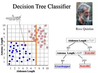
Decision Tree Classifier. 10. 9. 8. 7. 6. 5. 4. 3. 2. 1. 1. 2. 3. 4. 5. 6. 7. 8. 9. 10. Ross Quinlan. Abdomen Length > 7.1?. Antenna Length. yes. no. Antenna Length > 6.0?. Katydid. yes. no. Katydid. Grasshopper. Abdomen Length. Antennae shorter than body?.

Decision Tree Classifier
E N D
Presentation Transcript
Decision Tree Classifier 10 9 8 7 6 5 4 3 2 1 1 2 3 4 5 6 7 8 9 10 Ross Quinlan Abdomen Length > 7.1? Antenna Length yes no Antenna Length > 6.0? Katydid yes no Katydid Grasshopper Abdomen Length
Antennae shorter than body? Yes No 3 Tarsi? Grasshopper Yes No Foretiba has ears? Yes No Cricket Decision trees predate computers Katydids Camel Cricket
Decision Tree Classification • Decision tree • A flow-chart-like tree structure • Internal node denotes a test on an attribute • Branch represents an outcome of the test • Leaf nodes represent class labels or class distribution • Decision tree generation consists of two phases • Tree construction • At start, all the training examples are at the root • Partition examples recursively based on selected attributes • Tree pruning • Identify and remove branches that reflect noise or outliers • Use of decision tree: Classifying an unknown sample • Test the attribute values of the sample against the decision tree
How do we construct the decision tree? • Basic algorithm (a greedy algorithm) • Tree is constructed in a top-down recursive divide-and-conquer manner • At start, all the training examples are at the root • Attributes are categorical (if continuous-valued, they can be discretized in advance) • Examples are partitioned recursively based on selected attributes. • Test attributes are selected on the basis of a heuristic or statistical measure (e.g., information gain) • Conditions for stopping partitioning • All samples for a given node belong to the same class • There are no remaining attributes for further partitioning – majority voting is employed for classifying the leaf • There are no samples left
Information Gain as A Splitting Criteria • Select the attribute with the highest information gain (information gain is the expected reduction in entropy). • Assume there are two classes, P and N • Let the set of examples S contain p elements of class P and n elements of class N • The amount of information, needed to decide if an arbitrary example in S belongs to P or N is defined as 0 log(0) is defined as0
Information Gain in Decision Tree Induction • Assume that using attribute A, a current set will be partitioned into some number of child sets • The encoding information that would be gained by branching on A Note: entropy is at its minimum if the collection of objects is completely uniform
Entropy(4F,5M) = -(4/9)log2(4/9) - (5/9)log2(5/9) = 0.9911 no yes Hair Length <= 5? Let us try splitting on Hair length Entropy(3F,2M) = -(3/5)log2(3/5) - (2/5)log2(2/5) = 0.9710 Entropy(1F,3M) = -(1/4)log2(1/4) - (3/4)log2(3/4) = 0.8113 Gain(Hair Length <= 5) = 0.9911 – (4/9 * 0.8113 + 5/9 * 0.9710 ) = 0.0911
Entropy(4F,5M) = -(4/9)log2(4/9) - (5/9)log2(5/9) = 0.9911 no yes Weight <= 160? Let us try splitting on Weight Entropy(0F,4M) = -(0/4)log2(0/4) - (4/4)log2(4/4) = 0 Entropy(4F,1M) = -(4/5)log2(4/5) - (1/5)log2(1/5) = 0.7219 Gain(Weight <= 160) = 0.9911 – (5/9 * 0.7219 + 4/9 * 0 ) = 0.5900
Entropy(4F,5M) = -(4/9)log2(4/9) - (5/9)log2(5/9) = 0.9911 no yes age <= 40? Let us try splitting on Age Entropy(1F,2M) = -(1/3)log2(1/3) - (2/3)log2(2/3) = 0.9183 Entropy(3F,3M) = -(3/6)log2(3/6) - (3/6)log2(3/6) = 1 Gain(Age <= 40) = 0.9911 – (6/9 * 1 + 3/9 * 0.9183 ) = 0.0183
Of the 3 features we had, Weight was best. But while people who weigh over 160 are perfectly classified (as males), the under 160 people are not perfectly classified… So we simply recurse! no yes Weight <= 160? This time we find that we can split on Hair length, and we are done! no yes Hair Length <= 2?
We need don’t need to keep the data around, just the test conditions. Weight <= 160? yes no How would these people be classified? Hair Length <= 2? Male yes no Male Female
It is trivial to convert Decision Trees to rules… Weight <= 160? yes no Hair Length <= 2? Male no yes Male Female Rules to Classify Males/Females IfWeightgreater than 160, classify as Male Elseif Hair Lengthless than or equal to 2, classify as Male Else classify as Female
Once we have learned the decision tree, we don’t even need a computer! This decision tree is attached to a medical machine, and is designed to help nurses make decisions about what type of doctor to call. Decision tree for a typical shared-care setting applying the system for the diagnosis of prostatic obstructions.
The worked examples we have seen were performed on small datasets. However with small datasets there is a great danger of overfitting the data… When you have few datapoints, there are many possible splitting rules that perfectly classify the data, but will not generalize to future datasets. Yes No Wears green? Male Female For example, the rule “Wears green?” perfectly classifies the data, so does “Mothers name is Jacqueline?”, so does “Has blue shoes”…
PSA = serum prostate-specific antigen levels PSAD = PSA density TRUS = transrectal ultrasound Garzotto M et al. JCO 2005;23:4322-4329
Avoid Overfitting in Classification • The generated tree may overfit the training data • Too many branches, some may reflect anomalies due to noise or outliers • Result is in poor accuracy for unseen samples • Two approaches to avoid overfitting • Prepruning: Halt tree construction early—do not split a node if this would result in the goodness measure falling below a threshold • Difficult to choose an appropriate threshold • Postpruning: Remove branches from a “fully grown” tree—get a sequence of progressively pruned trees • Use a set of data different from the training data to decide which is the “best pruned tree”
10 10 100 9 9 90 8 8 80 7 7 70 6 6 60 5 5 50 4 4 40 3 3 30 2 2 20 1 1 10 1 1 2 2 3 3 4 4 5 5 6 6 7 7 8 8 10 10 9 9 10 20 30 40 50 60 70 80 100 90 Which of the “Pigeon Problems” can be solved by a Decision Tree? • Deep Bushy Tree • Useless • Deep Bushy Tree ? The Decision Tree has a hard time with correlated attributes
Advantages/Disadvantages of Decision Trees • Advantages: • Easy to understand (Doctors love them!) • Easy to generate rules • Disadvantages: • May suffer from overfitting. • Classifies by rectangular partitioning (so does not handle correlated features very well). • Can be quite large – pruning is necessary. • Does not handle streaming data easily
Naïve Bayes Classifier Thomas Bayes 1702 - 1761 We will start off with a visual intuition, before looking at the math…
10 9 8 7 6 5 4 3 2 1 1 2 3 4 5 6 7 8 9 10 Grasshoppers Katydids Antenna Length Abdomen Length Remember this example? Let’s get lots more data…
10 9 8 7 6 5 4 3 2 1 1 2 3 4 5 6 7 8 9 10 Katydids Grasshoppers With a lot of data, we can build a histogram. Let us just build one for “Antenna Length” for now… Antenna Length
We can leave the histograms as they are, or we can summarize them with two normal distributions. Let us us two normal distributions for ease of visualization in the following slides…
We want to classify an insect we have found. Its antennae are 3 units long. How can we classify it? • We can just ask ourselves, give the distributions of antennae lengths we have seen, is it more probable that our insect is a Grasshopperor a Katydid. • There is a formal way to discuss the most probable classification… p(cj | d) = probability of class cj, given that we have observed d 3 Antennae length is 3
p(cj | d) = probability of class cj, given that we have observed d P(Grasshopper | 3 ) = 10 / (10 +2) = 0.833 P(Katydid | 3 ) = 2 / (10 + 2) = 0.166 10 2 3 Antennae length is 3
p(cj | d) = probability of class cj, given that we have observed d P(Grasshopper | 7 ) = 3 / (3 +9) = 0.250 P(Katydid | 7 ) = 9 / (3 + 9) = 0.750 9 3 7 Antennae length is 7
p(cj | d) = probability of class cj, given that we have observed d P(Grasshopper | 5 ) = 6 / (6 +6) = 0.500 P(Katydid | 5 ) = 6 / (6 + 6) = 0.500 6 6 5 Antennae length is 5
Bayes Classifiers • That was a visual intuition for a simple case of the Bayes classifier, also called: • Idiot Bayes • Naïve Bayes • Simple Bayes • We are about to see some of the mathematical formalisms, and more examples, but keep in mind the basic idea. • Find out the probability of the previously unseen instance belonging to each class, then simply pick the most probable class.
Bayes Classifiers • Bayesian classifiers use Bayes theorem, which says p(cj | d ) = p(d | cj ) p(cj) p(d) • p(cj | d) = probability of instance d being in class cj, This is what we are trying to compute • p(d | cj) = probability of generating instance d given class cj, We can imagine that being in class cj, causes you to have feature d with some probability • p(cj) = probability of occurrence of class cj, This is just how frequent the class cj, is in our database • p(d) = probability of instance d occurring This can actually be ignored, since it is the same for all classes
(Note: “Drew can be a male or female name”) Drew Barrymore Assume that we have two classes c1 = male, and c2 = female. We have a person whose sex we do not know, say “drew” or d. Classifying drew as male or female is equivalent to asking is it more probable that drew is male or female, I.e which is greater p(male| drew) or p(female| drew) Drew Carey What is the probability of being called “drew” given that you are a male? What is the probability of being a male? p(male| drew) = p(drew | male) p(male) p(drew) What is the probability of being named “drew”? (actually irrelevant, since it is that same for all classes)
This is Officer Drew (who arrested me in 1997). Is Officer Drew a Male or Female? Luckily, we have a small database with names and sex. We can use it to apply Bayes rule… Officer Drew p(cj | d) = p(d | cj ) p(cj) p(d)
p(cj | d) = p(d | cj ) p(cj) p(d) Officer Drew p(male| drew) = 1/3 * 3/8 = 0.125 3/83/8 Officer Drew is more likely to be a Female. p(female| drew) = 2/5 * 5/8 = 0.250 3/83/8
Officer Drew IS a female! Officer Drew p(male| drew) = 1/3 * 3/8 = 0.125 3/8 3/8 p(female| drew) = 2/5 * 5/8 = 0.250 3/8 3/8
So far we have only considered Bayes Classification when we have one attribute (the “antennae length”, or the “name”). But we may have many features. How do we use all the features? p(cj | d) = p(d | cj ) p(cj) p(d)
To simplify the task, naïve Bayesian classifiers assume attributes have independent distributions, and thereby estimate p(d|cj) = p(d1|cj) * p(d2|cj) * ….* p(dn|cj) The probability of class cj generating instance d, equals…. The probability of class cj generating the observed value for feature 1, multiplied by.. The probability of class cj generating the observed value for feature 2, multiplied by..
To simplify the task, naïve Bayesian classifiers assume attributes have independent distributions, and thereby estimate p(d|cj) = p(d1|cj) * p(d2|cj) * ….* p(dn|cj) • p(officer drew|cj) = p(over_170cm = yes|cj) * p(eye =blue|cj) * …. Officer Drew is blue-eyed, over 170cm tall, and has long hair • p(officer drew| Female) = 2/5 * 3/5 * …. • p(officer drew| Male) = 2/3 * 2/3 * ….
cj The Naive Bayes classifiers is often represented as this type of graph… Note the direction of the arrows, which state that each class causes certain features, with a certain probability p(d1|cj) p(d2|cj) p(dn|cj) …
cj Naïve Bayes is fast and space efficient We can look up all the probabilities with a single scan of the database and store them in a (small) table… p(d1|cj) p(d2|cj) p(dn|cj) …
Naïve Bayes is NOT sensitive to irrelevant features... Suppose we are trying to classify a persons sex based on several features, including eye color. (Of course, eye color is completely irrelevant to a persons gender) • p(Jessica |cj) = p(eye = brown|cj) * p( wears_dress = yes|cj) * …. • p(Jessica | Female) = 9,000/10,000 * 9,975/10,000 * …. • p(Jessica | Male) = 9,001/10,000 * 2/10,000 * …. Almost the same! However, this assumes that we have good enough estimates of the probabilities, so the more data the better.
cj An obvious point. I have used a simple two class problem, and two possible values for each example, for my previous examples. However we can have an arbitrary number of classes, or feature values p(d1|cj) p(d2|cj) p(dn|cj) …
Problem! Naïve Bayes assumes independence of features… p(d|cj) Naïve Bayesian Classifier p(d1|cj) p(d2|cj) p(dn|cj)
Solution Consider the relationships between attributes… p(d|cj) Naïve Bayesian Classifier p(d1|cj) p(d2|cj) p(dn|cj)
Solution Consider the relationships between attributes… p(d|cj) Naïve Bayesian Classifier p(d1|cj) p(d2|cj) p(dn|cj) But how do we find the set of connecting arcs??
The Naïve Bayesian Classifierhas a quadratic decision boundary 10 9 8 7 6 5 4 3 2 1 1 2 3 4 5 6 7 8 9 10
Dear SIR, I am Mr. John Coleman and my sister is Miss Rose Colemen, we are the children of late Chief Paul Colemen from Sierra Leone. I am writing you in absolute confidence primarily to seek your assistance to transfer our cash of twenty one Million Dollars ($21,000.000.00) now in the custody of a private Security trust firm in Europe the money is in trunk boxes deposited and declared as family valuables by my late father as a matter of fact the company does not know the content as money, although my father made them to under stand that the boxes belongs to his foreign partner. …
This mail is probably spam. The original message has been attached along with this report, so you can recognize or block similar unwanted mail in future. See http://spamassassin.org/tag/ for more details. Content analysis details: (12.20 points, 5 required) NIGERIAN_SUBJECT2 (1.4 points) Subject is indicative of a Nigerian spam FROM_ENDS_IN_NUMS (0.7 points) From: ends in numbers MIME_BOUND_MANY_HEX (2.9 points) Spam tool pattern in MIME boundary URGENT_BIZ (2.7 points) BODY: Contains urgent matter US_DOLLARS_3 (1.5 points) BODY: Nigerian scam key phrase ($NN,NNN,NNN.NN) DEAR_SOMETHING (1.8 points) BODY: Contains 'Dear (something)' BAYES_30 (1.6 points) BODY: Bayesian classifier says spam probability is 30 to 40% [score: 0.3728]
Advantages/Disadvantages of Naïve Bayes • Advantages: • Fast to train (single scan). Fast to classify • Not sensitive to irrelevant features • Handles real and discrete data • Handles streaming data well • Disadvantages: • Assumes independence of features
Summary of Classification • We have seen 4 major classification techniques: • Simple linear classifier, Nearest neighbor, Decision tree. • There are other techniques: • Neural Networks, Support Vector Machines, Genetic algorithms.. • In general, there is no one best classifier for all problems. You have to consider what you hope to achieve, and the data itself… Let us now move on to the other classic problem of data mining and machine learning, Clustering…