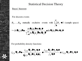
Statistical Decision Theory, Bayes Classifier
250 likes | 505 Vues
Statistical Decision Theory, Bayes Classifier. Lecture Notes for CMPUT 466/551 Nilanjan Ray. Supervised Learning Problem. Input (random) variable: X Output (random) variable: Y. A toy example:. unknown. A set of realizations of X and Y are available in (input, output) pairs:.

Statistical Decision Theory, Bayes Classifier
E N D
Presentation Transcript
Statistical Decision Theory,Bayes Classifier Lecture Notes for CMPUT 466/551 Nilanjan Ray
Supervised Learning Problem Input (random) variable: X Output (random) variable: Y A toy example: unknown A set of realizations of X and Y are available in (input, output) pairs: This set T is known as the training set Supervised Learning Problem: given the training set, we want to estimate the value of the output variable Y for a new input variable value, X=x0 ? Essentially here we try to learn the unknown function f from T.
Basics of Statistical Decision Theory We want to attack the supervised learning problem from the viewpoint of probability and statistics. Thus, let’s consider X and Y as random variables with a joint probability distribution Pr(X,Y). Assume a loss function L(Y,f(x)), such as a squared loss (L2): Choose f so that the expected prediction error is minimized: Known as regression function Also known as (non-linear) filtering in signal processing The minimizer is the conditional expectation : So, if we knew Pr(Y|X), we would readily estimate the output See [HTF] for the derivation of this minimization; Also see [Bishop] for a different derivation– know about a heavier machinery, called calculus of variations
Loss Functions and Regression Functions L1 loss: RF is conditional median: 0-1 loss: RF is conditional mode: Used in boosting… Exponential loss function Robust to outliers… Huber loss function Own student award in … Your loss function Observation: the estimator/regression function is always defined in terms of the conditional probability Pr(Y|X) Pr(Y|X) is Typically unknown to us, so what can we do??
Create Your Own World • Example Strategies: • Try to estimate regression function directly from training data • Assume some models, or structure on the solution,….so that the EPE minimization becomes tractable • Your own award winning paper • Etc… Structure free Highly structured
Nearest-Neighbor Method Use those observations to predict that are neighbors of the (new) input: Nk(x) is the neighborhood of x defined by k-closest points xi in the training sample Estimates the regression function directly from the training set: Nearest neighbor method is also (traditionally) known as a nonparametric method
Nearest-Neighbor Fit • Major limitations: • Very in inefficient in high dimension • Could be unstable (wiggly) • If training data is scarce, may not be the right choice For data description see [HTF], Section 2.3.3
How to Choose k: Bias-Variance Trade-off Let’s try to answer the obvious question: how can we choose k? One way to get some insight about k is the bias-variance trade-off Let’s say input-output model is Test error: Irreducible error (the regressor has no control) Will decrease as k increases Will most likely increase as k increases So we can find a trade-off between bias and variance to choose k
Bias Variance Trade-off Bias variance trade-off: Graphical representation
Assumption on Regression Function: Linear Models Structural assumption: Output Y is linear in the inputs X=(X1, X2, X3,…, Xp) Predict the output by: Vector notation, 1 included in X We estimate β from the training set (by least square): Can be shown that EPE minimization leads to this estimate with the linear model (see the comments in [HTF] section 2.4) Where, So, for a new input The regression output is
Example of Linear Model Fit Classification rule: Very stable (not wiggly), and computationally efficient. However, if the linear model assumption fails, the regression fails miserably X2 X1 X = (X1, X2) Y = (Red, Green), coded as Red=1, Green=0
More Regressors • Many regression techniques are based on modifications of linear models and nearest-neighbor techniques • Kernel methods • Local regression • Basis expansions • Projection pursuits and neural networks • …. Chapter 2 of [HTF] gives their quick overview
Bayes Classifier The key probability distribution Pr(Y|X) in the Bayesian paradigm called posterior distribution EPE is also called Risk in the Bayesian terminology; however Risk is more general than EPE We can show that EPE is the average error of classification under 0-1 penalty in the Risk So the Bayes’ classifier is minimum error classifier Corresponding error is called Bayes’ risk / Bayes rate etc. Materials mostly based on Ch 2 of [DHS] book
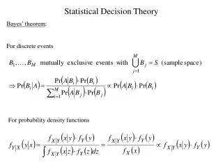
R1 R2 R3 R1 Bayes’ Classifier… We can associate probabilities to the categories (output classes) of the classifier This probability is called prior probability or simply the prior We assign a cost (Cij) to each possible decision outcome: Hi is true, we choose Hj M=3 2D input space, X We know the conditional probability densities p(X|Hi) Also called likelihood of the hypothesis Hi, or simply the likelihood Total risk
Bayes’ Classifier… Choose the Rj’s in such as way that this risk is minimized Since Rj partitions the entire region, any x will belong to exactly one such Rj So we can minimize the risk via the following rule to construct the partitions: You should realize that the reasoning is similar to that in [HTF] while minimizing EPE in Section 2.4.
Minimum Error Criterion 0-1 criterion: We are minimizing the Risk with 0-1 criterion This is also known as minimum error criterion In this case the total risk is the probability of error Note that Posterior probability This is same result if you minimize the EPE with 0-1 loss function (see [HTF] Section 2.4)
Two Class Case: Likelihood Ratio Test We can write Risk as: We can immediately see the rule of classification from above: Assign x to H1 if else assign x to H2 Likelihood ratio Special case: 0-1 criterion
An Example: Bayes Optimal Classifier We exactly know the posterior distribution of the two distribution, from which these boundaries are created
Minimax Classification Bayes rule: In many real life applications, prior probabilities may be unknown So we cannot have a Bayes’ optimal classification. However, one may wish to minimize the worst case overall risk We can write the Risk as a function of P1 and R1: Observation 1: If we fix R1 then Risk is a linear function of P1 Observation 2: The function is concave in P1
Minimax… Let’s arbitrarily fix P1 = a, and compute By observation 1, is the straight line AB Q: why should it be a tangent to g(P1)? is not a good classification when P1 is not known. Why? Claim: So, what could be a better classification here? The classification corresponding to MN. Why? This is the minimax solution Why the name? We can reach the solution by An aside Q: when can we reverse the order and get the same result? Another way to solve R1 in minimax is from: If you get multiple solutions, choose one that gives you the minimum Risk
Neyman-Pearson Criterion Consider a two class problem Following four probabilities can be computed: Probability of detection (hit) Probability of false alarm Probability of miss Probability of correct rejection R2 R1 We do not know the prior probabilities, so Bayes’s optimum classification is not possible However we do know that Probability of False alarm must be below Based on this constraint (Neyman-Pearson criterion) we can design a classifier Observation: maximizing probability of detection and minimizing probability of false alarm are conflicting goals (in general)
Receiver Operating Characteristics ROC is a plot: probability of false alarm vs. probability of detection Classifier 1 Probability of detection Classifier 2 Probability of false alarm Area under ROC curve is a measure of performance Used also to find a operating point for the classifier