Download
1 / 36
360 likes | 378 Vues
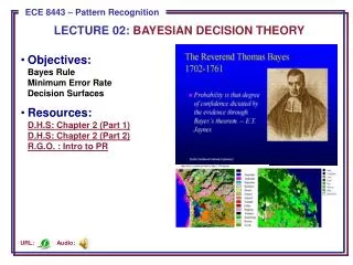
This text discusses Bayesian decision theory and its differences from classical approaches in statistical decision theory. It covers concepts such as prior density, likelihood, posterior density, and decision-theoretic elements. Examples and applications are provided to illustrate the use of Bayesian procedures in decision-making.

E N D
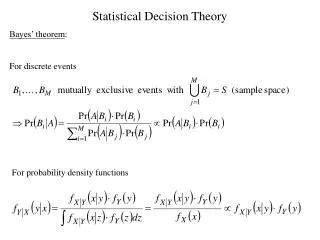
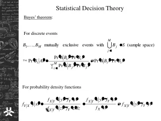
Statistical Decision Theory Bayes’ theorem: For discrete events For probability density functions
The Bayesian “philosophy” The classical approach (frequentist’s view): The random sample X = (X1, … , Xn ) is assumed to come from a distribution with a probability density function f (x; ) where is an unknown but fixed parameter. The sample is investigated from its random variable properties relating to f (x; ) . The uncertainty about is solely assessed on basis of the sample properties.
The Bayesian approach: The random sample X = (X1, … , Xn ) is assumed to come from a distribution with a probability density function f (x; ) where the uncertainty about is modelled with a probability distribution (i.e. a p.d.f), called the prior distribution The obtained values of the sample, i.e. x = (x1, … , xn ) are used to update the information from the prior distribution to a posterior distribution for Main differences: In the classical approach, is fix, while in the Bayesian approach is a random variable. In the classical approach focus is on the sampling distribution of X, while in the Bayesian the sample focus is on the variation of . • Bayesian: “What we observe is fixed, what we do not observe is random.” • Frequentist: “What we observe is random, what we do not observe is fixed.”
Concepts of the Bayesian framework Prior density: p( ) Likelihood: L( ; x) “as before” Posterior density: q( | x ) = q( ; x ) The book uses the second notation Relation through Bayes’ theorem:
The textbook writes Still the posterior is referred to as the distribution of conditional onx
Decision-theoretic elements • One of a number of actions should be decided on. • State of nature: A number of states possible. Usually represented by • For each state of nature the relative desirability of each of the different actions possible can be quantified • Prior information for the different states of nature may be available: Prior distribution of • Datamay be available. Usually represented by x. Can be used to update the knowledge about the relative desirability of (each of) the different actions.
In mathematical notation for this course: True state of nature: Uncertainty described by the prior p ( ) Data: xobservation of X, whose p.d.f. depends on (data is thus assumed to be available) Decision procedure: Action: (x) The decision procedure becomes an action when applied to given datax Loss function: LS ( , (x) ) measures the loss from taking action (x) when holds Risk function
Note that the risk function is the expected loss with respect to the simultaneous distribution of X1, … , Xn Note also that the risk function is for the decision procedure, and not for the particular action Admissible procedures: A procedure 1 is inadmissible if there exists another procedure such that R( , 1 ) R( , 2 ) for all values of . A procedure which is not inadmissible (i.e. no other procedure with lower risk function for any can be found) is said to be admissible
Minimax procedure: A procedure * is a minimax procedure if i.e. is chosen to be the “worst” possible value, and under that value the procedure that gives the lowest possible risk is chosen The minimax procedure uses no prior information about , thus it is not a Bayesian procedure.
Example Suppose you are about to make a decision on whether you should buy or rent a new TV. 1 = “Buy the TV” 2 = “Rent the TV” Now, assume is the mean time until the TV breaks down for the first time Let assume three possible values 6, 12 and 24 months The cost of the TV is $500 if you buy it and $30 per month if you rent it If the TV breaks down after 12 months you’ll have to replace it for the same cost as you bought it if you bought it. If you rented it you will get a new TV for no cost provided you proceed with your contract. Let X be the time in months until the TV breaks down and assume this variable is exponentially distributed with mean A loss function for an ownership of maximum 24 months may be defined as LS ( , 1(X ) ) = 500 + 500 H (X – 12) and LS ( , 2(X ) ) = 30 24 = 720
Then Now compare the risks for the three possible values of Clearly the risk for the first procedure increases with while the risk for the second in constant. In searching for the minimax procedure we therefore focus on the largest possible value of where 2 has the smallest risk 2 is the minimax procedure
Bayes procedure Bayes risk: Uses the prior distribution of the unknown parameter A Bayes procedure is a procedure that minimizes the Bayes risk
Example cont. Assume the three possible values of (6, 12 and 24) has the prior probabilities 0.2, 0.3 and 0.5. Then Thus the Bayes risk is minimized by 1 and therefore 1 is the Bayes procedure
Decision theory applied on point estimation The action is a particular point estimator State of nature is the true value of The loss function is a measure of how good (desirable) the estimator is of : Prior information is quantified by the prior distribution (p.d.f.) p( ) Data is the random sample x from a distribution with p.d.f. f (x ; )
Three simple loss functions Zero-one loss: Absolute error loss: Quadratic (error) loss:
Minimax estimators: Find the value of that maximizes the expected loss with respect to the sample values, i.e. that maximizes Then, the particular estimator that minimizes the risk for that value of is the minimax estimator Not so easy to find!
Bayes estimators A Bayes estimator is the estimator that minimizes For any given value of x what has to be minimized is
The Bayes philosophy is that data (x ) should be considered to be given and therefore the minimization cannot depend on x. Now minimization with respect to different loss functions will result in measures of location in the posterior distribution of . Zero-one loss: Absolute error loss: Quadratic loss:
About prior distributions Conjugate prior distributions Example: Assume the parameter of interest is , the proportion of some property of interest in the population (i.e. the probability for this property to occur) A reasonable prior density for is the Beta density:
Now, assume a sample of size n from the population in which y of the values possess the property of interest. The likelihood becomes Thus, the posterior density is also a Beta density with parameters y + and n – y +
Prior distributions that combined with the likelihood gives a posterior in the same distributional family are named conjugate priors. (Note that by a distributional family we mean distributions that go under a common name: Normal distribution, Binomial distribution, Poisson distribution etc. ) A conjugate prior always go together with a particular likelihood to produce the posterior. • We sometimes refer to a conjugate pair of distributions meaning • (prior distribution, sample distribution = likelihood)
In particular, if the sample distribution, i.e. f (x; ) belongs to the k-parameter exponential family of distributions: we may put where 1 , … , k + 1 are parameters of this prior distribution and K( )is a function of 1 , … , k + 1 only .
Then i.e. the posterior distribution is of the same form as the prior distribution but with parameters instead of
Some common cases: Conjugate prior Sample distribution Posterior Beta Binomial Beta Normal Normal, known 2 Normal Gamma Poisson Gamma Pareto Uniform Pareto
Example Assume we have a sample x = (x1, … , xn ) from U (0, ) and that a prior density for is the Pareto density What is the Bayes estimator of under quadratic loss? The Bayes estimator is the posterior mean. The posterior distribution is also Pareto with
Non-informative priors (uninformative) A prior distribution that gives no more information about than possibly the parameter space is called a non-informative or uninformative prior. Example: Beta(1,1) for an unknown proportion simply says that the parameter can be any value between 0 and 1 (which coincides with its definition) A non-informative prior is characterized by the property that all values in the parameter space are equally likely. Proper non-informative priors: The prior is a true density or mass function Improper non-informative priors: The prior is a constant value over Rk Example: N ( , ) for the mean of a normal population
Decision theory applied on hypothesis testing Test of H0: = 0 vs. H1: = 1 Decision procedure: C = Use a test with critical region C Action: C (x) = “Reject H0 if x C , otherwise accept H0 ” Loss function:
Risk function • Assume a prior setting p0 = Pr (H0 is true) = Pr ( = 0) and p1 = Pr (H1 is true) = Pr ( = 1) • The prior expected risk becomes
Bayes test: Minimax test: Lemma 6.1: Bayes tests and most powerful tests (Neyman-Pearson lemma) are equivalent in that every most powerful test is a Bayes test for some values of p0 and p1 and every Bayes test is a most powerful test with
Example: Assume x = (x1, x2 ) is a random sample from Exp( ), i.e. We would like to test H0: =1 vs. H0: =2 with a Bayes test with losses a = 2 and b = 1 and with prior probabilities p0 and p1
Now, A fixed size gives conditions on p0 and p1, and a certain choice will give a minimized
Sequential probability ratio test (SPRT) Suppose that we consider the sampling to be the observation of values in a “stream” x1, x2, … , i.e. we do not consider a sample with fixed size. We would like to test H0: = 0 vs. H1: = 1 After n observations have been taken we have xn= (x1, … , xn ) , and we put as the current test statistic.
The frequentist approach: Specify two numbers K1 and K2 not depending on n such that 0 < K1 < K2 < . Then If LR(n) K1 Stop sampling, accept H0 If LR(n) K2 Stop sampling, reject H0 If K1 < LR(n) < K2 Take another observation Usual choice of K1 and K2 (Property 6.3): If the size and the power 1 – are pre-specified, put This gives approximate true size and approximate true power 1 –
The Bayesian approach: The structure is the same, but the choices of K1 and K2 is different. Let c be the cost of taking one observation, and let as before a and b be the loss values for taking the wring decisions, and p0 and p1 be the prior probabilities of H0 and H1 respectively. Then the Bayesian choices of K1and K2 are