Download
1 / 115
1.16k likes | 1.55k Vues
DESIGN OF ROBUST CONTROL SYSTEM FOR A PARAMETRIC UNCERTAIN JET ENGINE POWER PLANT. Prof. P.S.V. Nataraj Systems & Control Engineering Indian Institute of Technology Bombay Mumbai, India. Overview. Introduction to Jet Engine Various Gas Turbine Configurations

E N D
DESIGN OF ROBUST CONTROL SYSTEM FOR A PARAMETRIC UNCERTAIN JET ENGINE POWER PLANT Prof. P.S.V. Nataraj Systems & Control Engineering Indian Institute of Technology Bombay Mumbai, India
Overview • Introduction to Jet Engine • Various Gas Turbine Configurations • Performance and Control of Turbojet Gas Turbine Engine • Control Requirements of aero Gas Turbine • Design Steps for the ControllerDesign • Robust Control Design Techniques
FUNDAMENTALS • For an aircraft turbine engine, it is necessary to achieve maximum thrust with minimum engine weight. • Control system should ensure all components operate at mechanical or thermal limits for at least one of the engine’s critical operating conditions.
FUNDAMENTALS …Cont. • Single input single output controls are used on commercial engines where emphasis is on economic operation. • Multivariable controls provide enhanced performance for military engines especially those with variable flow path geometry. • In both case the maximum use of the available performance within the structural and aero-thermal limitations is required.
Reheat burners Compressor Variable Geometry ( VG) Nozzle actuators Main Burners Afterburner flow Distributor Reheat Nozzle Hydromec-hanical Systems MainFuel VG Manual Fuel Control Linkage Fuel in PLA Gearbox Digital Electronic Control Unit Engine & System Feedback back JET ENGINE WITH INTEGRATED CONTROLS 7
Thrust Augmentation By Afterburning • Afterburner accomplishes short period increase in the rated thrust of the gas turbine engine • Objective is to improve the take off, climb and maximum speed characteristics of jet propelled aircraft
Various Gas Turbine Configurations • A Single Spool Turbojet Power Plant consists of an intake, a compressor, a combustion chamber, a turbine and a propelling nozzle. • A Twin Spool turbofan power plant consists of an intake, a low pressure compressor, high pressure compressor, a combustion chamber, a high pressure turbine, a low pressure turbine, a mixer, and a propelling nozzle.
Dynamic Performance of Turbojet Engine • Dynamic equations are obtained using the power balance, continuity and energy equations. • The steady state power balance equation simply implies that the power output of the turbine must equal the power absorbed by the compressor.
Control System Design • The increased gas turbine engine complexity has resulted in a corresponding increase in the complexity of the control system. • Control requirements applied to gas turbine engines consist of ensuring safe, stable engine operation. • An accurate and reliable control system is required to ensure needed engine performance and operational stability throughout the flight envelope. …Cont.
Control System Design …Cont. • The control system must sense Pilot’s commands, air frame requirements as well as critical engine parameters. • It must then compute the necessary schedules and actuate system variable for total engine control over the full range of operation. • Full authority digital electronic control system consists of two controllers, one of which is the digital electronic computer section and the other the back-up hydro mechanical section.
Control Requirements of aero Gas Turbine Engine • Relationship between the fuel flow control variable and the engine rotational speed over the flight envelope. • Relationship between the fuel flow control variable and the engine compression ratio over the flight envelope. • Relationship between the Power lever angle input into the control system and the rotational speed of the engine so as to incorporate a governing action and control engine thrust. ….Cont.
Control Requirements of Aero Gas Turbine Engine …Cont. • Set limits on fuel flows so as to ensure safe operation of engine without excess rotational speeds, temperatures and pressures at specific stations of the engine. • Position control of exhaust nozzle as per nozzle control schedule depending on Power Lever Angle (PLA) position. • Reheat fuel flow selection by Pilot through PLA.
Control Structure of Military Jet Engine
Design Steps for the Controller of Jet Engine • Selection of the basic operating requirements for each element of control. • Evaluation of engine requirements and control variables to select the mode of control that will provide the best operation. • Selection of types of control regulators and computing system . • Evaluation of stability requirements and basic performance requirements of the system
Design Steps for the Controller of Jet Engine …Cont. • Establishing the ability of the control components to meet the physical requirements of endurance, environment and vibration. • Evaluating the final system by analysis or testing to establish its ability to perform as required under actual operating conditions
Digital Control of Jet Engine • The primary control objectives of gas turbine i.e., thrust, is a complex and non-linear function of flight conditions like altitude, mach number and control variables comprising of main enginefuel flow, reheat fuel flow and nozzle area. • These parameters are to be controlled with complex schedules to a high accuracy. …Cont.
Digital Control of Jet Engine …Cont. • Full authority digital engine control system executes these schedules to provide the most optimum performance. • The control system components are the hydro mechanical fuel management units with built in pumps, metering values and position feedback transducers and nozzle control system and their corresponding digital control units.
MAJOR CONTROL LOOPS OF JET ENGINE POWER PLANT • HIGH PRESSURE COMPRESSOR ACCELERATION CONTROL LOOP • LOW PRESSURE COMRESSOR SPEED CONTROL LOOP • VARIABLE GEOMETRY CONTROL LOOP • NOZZLE CONTROL LOOP • AFTERBURNER FUEL FLOW CONTROL LOOP
MAIN FUEL FLOW CONTROLS NL • COMPRESSOR VARIABLE GEOMETRY CONTROLS NH • NOZZLE AREA SCHEDULED AS FUNCTION OF ALTITUDE AND PILOT THROTTLE POSITION • AFTERBURNER FUEL FLOW SCHEDULED AS A FUNCTION OF NOZZLE AREA AND ALTITUDE
BLOCK DIAGRAM OF HIGH PRESSURE COMPRESSOR SPEED ACCELERATION LOOP OF JET ENGINE
* 3 Parametric uncertainties in Plant. • * Uncertainty %: 5 % • Performance requirements for the inner • Acceleration loop: • 1. Stability Margins : Gain Margin = 6 dB; • Phase Margin = 450; • 2. Tracking Specifications : Rise time of closed loop transfer • function between 0.4 to 0.8 sec • 1. No overshoot
BLOCK DIAGRAM OF THE LOW PRESSURE COMPRESSOR SPEED CONTROL OF JET ENGINE
* 5 Parametric uncertainties in Plant. * Uncertainty %: 5 % Performance requirements for the outer Speed loop: 1. Stability Margins : Gain Margin = 6 dB; Phase Margin = 450; 2. Tracking Specifications : Rise time of closed loop transfer function between 0.7 to 0.95 sec 1. No overshoot
Nozzle Electro Hydromechanical System Demanded Nozzle Area Desired Actuator stroke Throttle Area to stroke converter Operating schedule Servo valve Controller Actuator Pump Temperature Actual Actuator stroke LVDT BLOCK DIAGRAM OF EXHAUST NOZZLE POSITION CONTROL SYSTEM Actuator position LVDT : Linear variable differential transducer (to measure stroke)
* 2 Parametric uncertainties in Plant. * Uncertainty %: 4 % Performance requirements for the Variable C Nozzle control loop: 1. Stability Margins : Gain Margin = 6 dB Phase Margin = 450 2. Tracking Specifications : Rise time of closed loop transfer function between 0.12 to 0.18 sec 1. No overshoot
BLOCK DIAGRAM OF AFTERBURNER FUEL FLOW CONTROL LOOP Demanded Afterburner Fuel flow Servo current Actual Afterburner fuel flow Throttle Operating schedule Afterburner H/M System Controller Temperature Operating Schedule : Afterburner fuel flow as a function of nozzle area
* 2 Parametric uncertainties in Plant. * Uncertainty %: 4 % Performance requirements for the Afterburner fuel flow control loop: 1. Stability Margins : Gain Margin = 6 dB; Phase Margin = 450; 2. Tracking Specifications : Rise time of closed loop transfer function between 0.55 to 0.78 sec 1. No overshoot
BLOCK DIAGRAM OF THE VARIABLE GEOMETRY CONTROL SYSTEM OF JET ENGINE POWER PLANT VG : Variable geometry IGV : Inlet guide vane H/M : Hydromechanical Pilot Throttle Desired Compressor IGV position + Operating schedule VG H/M System Compensator - Inlet Temperature Actual IGV position Input to VG H/M system : Servo valve current Output of VG H/M system : IGV Actuator Position
* 3 Parametric uncertainties in Plant. * Uncertainty %: 4 % Performance requirements for the variable Geometry control loop: 1. Stability Margins : Gain Margin = 6 dB; Phase Margin = 450; 2. Tracking Specifications : Rise time of closed loop transfer function between 0.15 to 0.24 sec 1. No overshoot
An Interval Analysis Approach for Design of Robust First Order Compensator for Jet Engine
Basic Concepts • Consider a strictly proper interval plant family P comprising of • plants of the form. • where interval bounds are a priori given for each uncertain coefficient qi and ri . Let C(s) be a compensator in a feedback structure for this interval plant. If C(s) is such that it stabilizes the entire P, then C(s) is said to robustly stabilize P. • If the compensator for an interval plant is first order, the stability of only sixteen extreme plants is necessary and sufficient to stabilize the entire interval family.
Block diagram of Compressor Speed control Loop of Jet Engine Desired Compressor Speed Throttle Operating Schedule Compressor Engine Inlet Temperature Compressor Speed
Block diagram of Ndot controller of Jet Engine Desired Ndot Ndot Schedule Inlet Temperature Compressor Engine Compressor Speed Differentiator
Algorithm for Compensator Synthesis Let 4 denote the set [1,2,3,4]. Let Ni1 (s) , i1 4 , denote the Kharitonov polynomials associated with NP(s,q). ….Cont.
Algorithm for Compensator Synthesis ..Cont. Consider that a robustly stabilizing PI controller is to be synthesized for an interval plant family P with Kharitonov’s polynomials N1 (s), N2 (s), N3 (s) and N4 (s) and D1 (s), D2 (s), D3 (s) and D4 (s) for the numerator and denominator respectively.
The sixteen extreme plants are defined by with i1, i2 {1,2,3,4}.
The compensator synthesis Algorithm given by Barmish et al. Algorithm: Synthesis of first order compensator (due to Barmish et. al.) Begin Algorithm (i) Set up sixteen Routh tables for closed loop polynomials associated with each extreme plant. (ii) Enforce positivity for each of the first column entries which are functions of K1 and K2. This leads to set of inequalities involving K1 and K2. (iii) To obtain the final controller, (K1, K2) should stabilize all sixteen extreme plants simultaneously. Let Ki1,i2, i1,i2 {1,2,3,4}
Denote the set of stabilizing gains corresponding to the i1th and i2th Kharitonov polynomial for the numerator and denominator, respectively. • Solve the inequalities for each of the sixteen extreme plants independently by gridding method and obtain the set of stabilizing gains for each of them. • (iv) Obtain the desired set of stabilising gains for the interval system as intersection of these results evaluated for the sixteen extreme plants. • END Algorithm.
Remarks • Here, the bounds for the stabilising gains are obtained in the selected range of K1 and K2. It is not possible to obtain all the solutions. Further, the results are guaranteed only at the gridding points. It may happen that a point between the selected grid points may not be a feasible solution. • The proposed algorithm using interval analysis evaluates the bounds for the stabilising gains, in which all feasible solutions are obtained as a set of interval boxes of specified accuracy. Any point within these interval box is a guaranteed stabilising gain for the interval system.
Algorithm: Synthesis of first order Compensator using interval analysis Begin Algorithm i) Obtained by replacing the gridding technique in step (iii) of Barmish et al’s algorithm given above with the sub-definite computations technique (to solve the set of inequalities involving the sixteen extreme plants). ii) Using sub-definite computation technique, obtain initial bounds on K1 and K2 in which all feasible solutions must lie. iii) Find all feasible solutions as interval boxes of specified accuracy in the initial bounds obtained at (ii) above. End Algorithm
Remark 1 The solution set obtained as a set of interval boxes contains all the feasible solutions. Any point within this box is a guaranteed stabilizing gain for the interval system. Remark 2 A necessary and sufficient condition for the existence of a robust stabilizing controller is non-emptiness of the set of gains in (iii) above. Remark 3 The interval plant P can be stabilized by selecting any (K1,K2) K.
A computer program has been developed for the above controller synthesis technique. • Consider the SISO Jet engine interval plant with input as fuel flow and output as acceleration of compressor speed, Ndot. • P(s,) = • The uncertainty bounds are • qo [940, 980], r1 [97, 107], r2 [215,230]
Let us synthesise a compensator of the form to stabilize the interval plant P(s,) The Kharitonov polynomials for the numerator and denominator of the effective plant of acceleration loop are: N1(s) = 940;N2(s) = 980; D1(s) = s2 + 97s + 215; D2(s) = s2 + 107s + 215; D3(s) = s2+107s+230; D4(s) = s2 + 97s + 230;
Thus, there are 8 different extreme plants. Using these extreme plants, and PI compensator C(s), the associated closed loop polynomials are derived as follows. p1,1(s) = s3 + 97s2 + (215+940K1)s + 940K2 p1,2(s) = s3 + 107s2 + (215+940K1)s + 940K2 p1,3(s) = s3 + 107s2 + (230 + 940K1)s + 940K2 p1,4,(s) = s3 + 97s2 + (230 + 940K1)s + 940K2 p3,1(s) = s3 + 97s2 + (215 + 980K1)s + 980K2 p3,2(s) = s3 + 107s2 + (215 + 980K1)s + 980K2 p3,3(s) = s3 + 107s2 + (230 + 940K1)s + 980K2 p3,4(s) = s3 + 97s2 + (230+980K1)s + 980K2
Routh table is set up for all the closed loop polynomials. • Inequalities associated with each closed loop polynomial are obtained. • These inequalities are solved using proposed interval analysis algorithm to obtain bounds on stabilizable controller parameters. • Any value within these bounds will stabilize the uncertain plant
Results obtained • 3 Inequalities associated with each closed loop polynomial • Thus 24 inequalities are solved using proposed interval analysis algorithm • Initial bounds on K1 and K2 are obtained as • [0, 2.19131e6] • Thus the given plant is stabilizable even with a very large value of K1 & K2 • However, large values of gain are not practical. • Practical gains can be obtained by implementing additional performance constraints.