Download
1 / 22
230 likes | 414 Vues
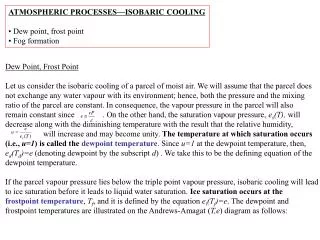
ATMOSPHERIC PROCESSES—ISOBARIC COOLING Dew point, frost point Fog formation. Dew Point, Frost Point Let us consider the isobaric cooling of a parcel of moist air. We will assume that the parcel does not exchange any water vapour with its environment; hence, both the pressure and the mixing

E N D
ATMOSPHERIC PROCESSES—ISOBARIC COOLING • Dew point, frost point • Fog formation Dew Point, Frost Point Let us consider the isobaric cooling of a parcel of moist air. We will assume that the parcel does not exchange any water vapour with its environment; hence, both the pressure and the mixing ratio of the parcel are constant. In consequence, the vapour pressure in the parcel will also remain constant since . On the other hand, the saturation vapour pressure, es(T), will decrease along with the diminishing temperature with the result that the relative humidity, will increase and may become unity. The temperature at which saturation occurs (i.e., u=1) is called the dewpoint temperature. Since u=1 at the dewpoint temperature, then, ed(Td)=e (denoting dewpoint by the subscript d) . We take this to be the defining equation of the dewpoint temperature. If the parcel vapour pressure lies below the triple point vapour pressure, isobaric cooling will lead to ice saturation before it leads to liquid water saturation. Ice saturation occurs at the frostpoint temperature, Tf, and it is defined by the equation ei(Tf)=e. The dewpoint and frostpoint temperatures are illustrated on the Andrews-Amagat (T,e) diagram as follows:
We can derive a relationship between the dewpoint depression, T-Td, and the relative humidity by integrating the Clausius-Clapeyron equation between points 1 and 2 on the diagram above. Assuming that over a small interval the latent heat of vapourization can be taken as a constant, and using the defining equation for the dewpoint temperature, the integration leads to: (13.1) Equation 13.1 may be written approximately as: (13.2)
where in Eq. 13.2, u is expressed as a fraction, not as a percent. As an example, if u=0.5 then T-Td=10.5 K. The fact that the dewpoint depression is a function of the relative humidity only, and not of the initial temperature, can be plainly seen be considering a few cases on the tephigram. Although thermodynamics can say that the air will be saturated at the dewpoint and frost points (with respect to liquid water and ice, respectively), it cannot say whether or not condensation or deposition will occur at these respective temperatures. Condensation and deposition at saturation will depend on the existence of suitable condensation or deposition nuclei (aerosol particles). In their absence, the air parcel will simply become supersaturated with water vapour if further cooling occurs. We can obtain a relation between the frostpoint and dewpoint temperatures by applying Eq. 13.1 between the triple point and point 3 on the diagram, and then again between the triple point and point 4 on the diagram, then subtracting the two equations. This leads to: (13.3) With temperatures written in oC, the last equality leads to: (13.4) It should be noted the Tf and Td are invariants under isobaric temperature changes of a closed air parcel.
FOG FORMATION (CONDENSATION BY ISOBARIC COOLING) When isobaric cooling of an air parcel results from loss of heat by radiation, a radiation fog forms at the dewpoint temperature. Further cooling causes the fog to “thicken” (I.e., the liquid water content in the fog increases). If the loss of heat occurs through heat transfer to a cold, underlying surface the resulting fog is called an advection fog. Both types of fog can be described with the same thermodynamics. As we will see, once a fog has formed, the release of latent heat substantially reduces the cooling rate with the result that the overnight minimum temperature with a radiation fog is often not much lower than the evening dewpoint temperature. We can calculate the “effective heat capacity” of foggy air as follows. For isobaric processes, q=dh, so for cloudy air: (13.5) We are seeking a relation between q and dT. Consequently, we need to establish a relation between drs and dT. This can be done using the Clausius-Clapeyron equation with p constant: (13.6)
(13.7) Substituting from Eq. 13.7 into Eq. 13.6 and thence into Eq. 13.5, we obtain the desired result: (13.8) The quantity in parentheses can be thought of as the isobaric “effective heat capacity” of foggy air. Clearly, it is higher than the isobaric specific heat capacity of dry air. Just how much higher can be demonstrated with an example. If saturated air at 25oC is cooled isobarically, its initial effective heat capacity is: cp=1.005x10³ Jkg-1 K-1 =0.622 lv=2.4418x10⁶ Jkg-1 (at 25oC) es=3.167x10³ Pa (at 25oC) p=105 kPa T=298.15 K Rv=4.6151x10² Jkg-1 K-1 and so:
This value is almost four times the isobaric specific heat capacity of dry air (almost as large, in fact, as the specific heat capacity of liquid water). Consequently, in this case, if the heat flux remains the same after fog formation, the rate of cooling of the air parcel will be reduced by a factor of almost four. -------------------------------------------------- Another question we might ask in connection with fog formation is, “How much liquid water condenses for a given temperature drop?” If c is the mass of liquid water per unit volume of the air parcel, and v is the vapour density, then conservation of mass requires that: (13.9) Differentiating the ideal gas law for water vapour at saturation, we have: (13.10) where the second term is much smaller that the first and may be neglected (the temperature squared term in the denominator dominates). Substituting for des in Eq. 13.10 from the Clausius-Clapeyron equation, and thence into Eq. 13.9, we have:
(13.11) As an example of the use of Eq. 13.11, we can ask what temperature change is required to produce a liquid water content of 1 gm-3 at 5oC and at 30oC. The results are shown in the table below: This example illustrates that a much bigger temperature change is required at low temperatures in order to obtain a fog of comparable liquid water content. This is why “dense” fogs tend to occur less frequently at low temperatures. However, one should keep in mind that the visibility in a fog of a particular liquid water content will depend on the drop size distribution. Reducing the volume median droplet diameter will also tend to reduce the visibility, even if the liquid water content remains the same. As an exercise, consider the above examples using the tephigram and check whether you get the same result. Take the pressure to be 100 kPa and the air density to be 1 kgm-3 , so that the liquid water content and the liquid water mixing ratio are the same.
ATMOSPHERIC PROCESSES—ADIABATIC/ISOBARIC • Isobaric equivalent temperature • Isobaric wet-bulb temperature • Psychrometric equation • Wind chill • Mixing fog Adiabatic, isobaric processes are isenthalpic since dh=q+vdp=0. For dry air, the result is uninteresting since dh=cpdT and isenthalpic processes are simply isothermal. Moist air, on the other hand, will cool if more water vapour is evaporated into it, or it will warm if water vapour condenses in it (keeping in mind that we have assumed adiabatic conditions, so that the latent heat must come from or be given to the air itself; i.e., the dry air/water vapour mix is adiabatic when taken together). With the possibility of phase changes in mind, we can substitute the latent heat release for q and write dh=cpdT+lvdr=0, with the result that cpT+lvr=const for such processes. Or, dividing by cp, then: (14.1) for adiabatic, isobaric processes.
ISOBARIC EQUIVALENT TEMPERATURE Suppose that it were possible to condense all the water vapour in an air parcel adiabatically and isobarically (actually, this is an impossible process but think of it as an hypothetical possibility). Then applying Eq. 14.1 to the initial and final states, we have: (14.2) where Tieis the isobaric equivalent temperature; that is, the temperature in the final, dry state following condensation of all the water vapour in the parcel (rie=0). Substituting values for the latent and specific heats, Eq. 14.2 becomes approximately Tie=T+2.5r, where r (in g/kg) is the actual mixing ratio of the air parcel. The isobaric equivalent temperature cannot be determined from the tephigram, although a related (and approximately equal) temperature can. This is the adiabatic equivalent temperature, which we shall encounter in two lectures (16). ISOBARIC WET-BULB TEMPERATURE Suppose water is evaporated into an air parcel, adiabatically and isobarically, until it is saturated. This is a physically realistic process. Examples include rain evaporating into the air below cloud base, and the wet-bulb thermometer. Once again, writing Eq. 14.1 for the initial and final states: (14.3)
where Tiw is the isobaric wet-bulb temperature, that is, the temperature of the air parcel after it has become saturated following the adiabatic, isobaric evaporation of water into it. The isobaric wet-bulb temperature is usually called simply the wet-bulb temperature, Tw. NOTES: 1) It should be noted that the isobaric wet-bulb temperature and the dew point temperature are achieved following very different physical processes. Hence they are not the same unless an air parcel is already saturated, in which case they are equal to each other as well as to the temperature of the air parcel. 2) Note that Eq. 14.3 is a non-linear equation in Tiw given the temperature dependence of the saturation mixing ratio. Hence, it must be solved numerically. An iterative process converges, in which one first estimates Tiw, and uses the estimate to evaluate rs(Tiw). Then Eq. 14.3 can be solved for a new estimate of Tiw, and the process repeated until the result changes little from iteration to iteration. PSYCHROMETRIC EQUATION Since the dew point temperature, Td, and the wet-bulb temperature, Tw, are both measures of the amount of water vapour in the air, they should be related to each other. This relation is called the psychrometric equation. It can be derived from Eq. 14.3, which can be re-arranged to give: (14.4) Using and the fact that e=es(Td), Eq. 14.4 becomes: (14.5)
Eq. 14.5 is the psychrometric equation. If we can measure T and Tw with a wet-bulb thermometer then we can use Eq. 14.5 to infer the dew-point temperature, Td. For some practical information regarding how to measure the wet-bulb temperature, see http://www.usatoday.com/weather/wsling.htm http://www.materialstestingequip.com/psychro.htm
Example Q: On the night of October 16, 1991, there was a wet snowfall in Edmonton. The pressure was 95 kPa. The following morning the temperature was 0oC and it was quite foggy. What were the initial temperature and mixing ratio of this air mass? A: Since it was foggy, we will assume a relative humidity of 100%. Hence, we infer that the wet-bulb temperature on the morning of October 17 was 0oC. Making use of our tephigram to determine rs, Eq. 14.3 then becomes: There is no unique answer for T and r. Several possibilities are listed below. Possibly the air mass passed through all of these states before becoming saturated. 10oC 0 g/kg 0% R.H. 5oC 2 g/kg 35% R.H. 2.5oC 3 g/kg 52% R.H.
It isn’t entirely obvious that a wet-bulb thermometer should indicate the isobaric, adiabatic wet-bulb temperature (the similarity of the names notwithstanding). We will demonstrate this as follows. Let the temperature measured by the wet-bulb thermometer be called T*. We will assume that it is in equilibrium with the airstream that is flowing past it, so that the evaporation from the wet gauze that surrounds the bulb is driven by the heat transfer from the airstream to the thermometer. The heat balance equation for this process (which we will derive later in conjunction with a discussion of hailstone thermodynamics) may be written: (14.6) where h is the heat transfer coefficient, Pr is the Prandtl number, Sc is the Schmidt number, u is the relative humidity, and T is the air temperature. (The Prandtl number is the ratio of momentum diffusivity to thermal diffusivity. The Schmidt number is the ratio of kinematic viscosity to molecular diffusivity.) Now the term involving the Prandtl and Schmidt numbers is approximately unity, and we can use the definitions of relative humidity and dewpoint temperature, viz.
Then Eq. 14.6 may be re-arranged to give: (14.7) If T*=Tw, then Eq. 14.7 is identical to the psychrometric equation (Eq. 14.5). Hence, we infer that the wet-bulb thermometer does indeed measure the isobaric wet-bulb temperature. The psychrometric equation suggests that adiabatic, isobaric processes can be represented as straight lines on an Andrews-Amagat diagram, as illustrated below: Note the position of the isobaric equivalent temperature, Tie (at zero vapour pressure) and its relation to T and es(Tw).
WIND CHILL INDEX The wind chill index is a measure of the heat flux from bare skin. The Edmonton weather office uses the following formula (courtesy of Brian Paruk, Jan. 1993): (14.8) where H is in Wm-2 , V is the wind speed in m/s, and T is the air temperature inoC. It is assumed that skin temperature is 33oC. Comparing Eq. 14.8 with the left hand side of Eq. 14.6, we see that the expression involving the wind speed gives the heat transfer coefficient. Note that Eq. 14.8 does not explicitly take into account evaporative cooling. Environment Canada has a website dedicated to the wind chill index, along with charts, graphs and a downloadable wind chill calculator: http://www.msc-smc.ec.gc.ca/education/windchill/index_e.cfm
MIXING FOG If we mix two air parcels isobarically and adiabatically, their final temperature and vapour pressure will be give approximately by the mass-weighted averages: (14.9) Thus the final point on an Andrews-Amagat diagram lies along a straight line joining the two air parcels, as in the diagrams below. Because of the downward curvature of the saturation vapour pressure curve, the mixed air parcel can have a higher relative humidity than either of the two original air parcels. In fact, it can be supersaturated. If there are condensation nuclei in the air, adiabatic, isobaric condensation in the supersaturated air parcel will occur along the psychrometric equation line (as in the diagram below), giving rise to an amount of condensed water given by Hence, the mixing of two initially unsaturated air parcels can cause a mixing fog. A common occurrence of such a fog is your visible breath when you exhale in wintertime. Another example is the condensation trail from jet aircraft.
ATMOSPHERIC PROCESSES—ADIABATIC EXPANSION • Moist adiabatic processes • Saturation temperature • Cloud base estimation Moist Adiabatic Processes Moist adiabatic expansion can be used to describe the thermodynamics of rising thermals, prior to the onset of condensation, under the assumption that there is no mixing with the environment (hence adiabatic). We will ignore the thermodynamic effect of the water vapour, so long as phase changes do not occur. Hence, we will approximate moist adiabatic expansion with dry adiabatic expansion which is described, very compactly, by Let us examine how the relative humidity changes during moist adiabatic expansion, with a view to the possibility that a rising thermal will eventually reach saturation. Differentiating, logarithmically, the definition of relative humidity (Eq. 8.23), we have: (15.1) We would like to express the RHS of Eq. 15.1 in terms of dT, since we know that a consequence of adiabatic expansion is a drop in temperature. Poisson’s equation for the vapour may be written as:
(15.2) Note: Eq. 15.2 is a consequence of Poisson’s equation Tp-=const and the fact that the mole fraction of the vapour remains constant since the air parcel is a closed system. That is, Nv=e/p=const. Alternatively, we may use the fact that the mixing ratio re/p=const, leading to the same result. We may logarithmically differentiate Eq. 15.2 and substitute into the first term on the RHS of Eq. 15.1. Then we may logarithmically differentiate the Clausius-Clapeyron equation and substitute into the second term on the RHS of Eq. 15.1. The result is: (15.3) which may be re-arranged to give: (15.4) Hence the relative humidity, u, will increase as the temperature of the adiabatically expanding air drops, provided T<lv/cp1500 K. This condition is always satisfied under meteorological conditions. Can you think of some dramatic examples where air temperature might exceed 1500 K and lead to saturation in air whose temperature is increasing?
SATURATION TEMPERATURE So we can be confident that if we continue to let our thermal rise adiabatically, the humidity will rise and it will eventually become saturated (u=1). We can find the saturation temperature, Ts, By integrating Eq. 15.3 between the initial point (T,u) and the final point (Ts,1): (15.5) This is a non-linear equation for Ts and it needs to be solved numerically. However, we can determine Ts quite easily using the tephigram. The sketch below indicates how this is done.
VARIATION OF DEW POINT UNDER MOIST ADIABATIC EXPANSION We can infer the height of the saturation point (i.e., the cloud base) by using the fact that the temperature and dewpoint temperature decline at different rates under moist adiabatic expansion. At the saturation point, however, they will be equal. This is illustrated in the sketches on the previous slide. As we will see later (and have already discovered from the tephigram), the dry adiabatic lapse rate is about 10oC/km. So let us determine the dewpoint temperature lapse rate. The Clausius-Clapeyron equation can be interpreted in terms of the dewpoint temperature as follows: (15.7) Substituting from Poisson’s equation (Eq. 15.2), logarithmically differentiated: (15.8) Hence, the lapse rate of the dewpoint temperature along a dry adiabat is approximately 1.7oC/km.
CLOUD BASE ESTIMATION If we know the initial temperature and the dewpoint temperature of a rising air parcel, we can estimate the height of the saturation point (the LIFTING CONDENSATION LEVEL or LCL), as follows. The temperature lapse rate between the initial point and the LCL is: (15.9) The dewpoint temperature lapse rate over the same interval is: (15.10) Combining Eqs. 15.9 and 15.10 leads to: (15.11) This formula will give the base of cumulus clouds which are formed by air rising undiluted from the level at which the temperature and dewpoint temperature are T and Td, respectively.