Download
1 / 78
790 likes | 1k Vues
A Comparison of Eight Economic Table Options. David Spring M.Ed., University of Washington Presentation to the Washington State Child Support Work Group December 14, 2007. Overview of Presentation. Introduction Overview of eight options

E N D
A Comparison of Eight Economic Table Options David Spring M.Ed., University of Washington Presentation to the Washington State Child Support Work Group December 14, 2007
Overview of Presentation Introduction • Overview of eight options • Drawbacks of over-estimating child support obligations • State and Federal Legal Requirements Problems with existing options • Concerns about the CEX and USDA per capita method. • Concerns about Engel and Betson-Rothbarth Indirect proxy methods • Concerns about the Rogers Cost Share method Two Additional Options • The Recommended Option: A Simplified Cost Share method • A Modified Status Quo Option (the New York model) Comparing 4 Options Simplified Cost Share Option compared to NY Model, the Current Table and the Betson-Rothbarth Model Cost Share Estimates for more than one child
11 Problem Solving Steps • Identify all reasonable options: avoid tunnel vision • Use multiple sources of information. • Analyze advantages and drawbacks of all options • Make implicit assumptions of each option explicit • Assess validity and reliability of all assumptions • Divide complex decisions into smaller decisions • Make explicit decisions on underlying assumptions before making bigger decisions. • Consider consequences of all options • Try to find a win-win solution: be flexible, consensus promotes cooperation • Sleep on it: snap decisions may not be good decisions • Choose the “most equitable” option for everyone.
Decision Making Questions Per capita or marginal child cost estimate? Direct cost or indirect proxy cost estimate? Bottom up detailed cost or top down total cost? Or a combination of bottom up and top down estimates? Assume child has two households or one? Is there a consistent relationship between spending patterns of: Couples with children and couples without children??? Intact families and non-intact families??? Rich, stable families and poor struggling families??? Spending on adult clothing and spending on children???
History Matters: Assumptions used to construct the current table The 1988 Washington State Child Support Guidelines were heavily influenced by Weitzman’s “math errors”. "Many Washington Courts set child support at amounts even lower than the inadequate and somewhat arbitrary schedule established by the Association of Superior Court Judges Uniform Child Support Guidelines. Lenore Weitzman and Ruth Dixon found that the amount of child support awarded in Los Angeles in 1972 was only half the amount needed to raise children in low income families.” (Divorce Reform and Child Support Guidelines,1987, pg 3). In 1996, Weitzman was finally forced to admit that her calculations were incorrect. Braver and O’Connell (1998) concluded that there was no statistically significant difference in the drop in standard of living between parents after divorce. Thus, the current Washington Economic Table is based upon assumptions and data that have since been shown to be false. Thus, there is a lack of trust in “experts.” It is notable that Weitzman’s downfall did not lead to a lowering of child support tables.
What is the basic assumption of “income shares” model? “The Income Shares Approach actually creates one normative statement, and it says What we should aim for, if possible, is to maintain the level of spending on the children to the level that would have occurred had the family remained intact… What I want to talk about today is if we agree with this normative statement how would we implement it?” Dr. David Betson, Child Support Work Group meeting, November 30, 2007 Thus, the goal of “income shares” is to maintain the level of spending on the child as if the family was still was still intact and living in one household. But what if we believe that intact-family spending patterns on children cannot be maintained after divorce?
What is the basic assumption of “income shares” model? “Clearly, those economies of scale are lost, when those families or their individuals split and form two new households. Which means that if the total amount of resources that are available to these two households remains exactly the same, one of them, at least one -- maybe both -- but at least one of those households has to be worse off in economic terms.” Dr. David Betson, Child Support Work Group meeting, November 30, 2007 Is the “income shares” assumption that the child only has one house and that all child expenses occur in only one household? Is the goal of “income shares” is to maintain the pre-divorce level of spending on the child only in the custodial parents house?
What is the basic assumption of the Washington State Parenting Act? “The State recognizes the fundamental importance of the parent/child relationship to the welfare of the child; and that the relationship between the child and each parent should be fostered unless inconsistent with the child’s best interest.”RCW 26.09.002 Washington State Law therefore assumes that the child will have two households after divorce and that the relationship between the child and each parent should be fostered. In other words, Washington State law assumes that the child will have two households after divorce and that both households are important to the child.
Washington State Legal Requirements RCW 26.19.001 states: The legislature intends, in establishing a child support schedule, to insure that child support orders are adequate to meet a child's basic needs and to provide additional child support commensurate with the parents' income, resources, and standard of living. The legislature also intends that the child support obligation should be equitably apportioned between the parents. The Betson model assumes that child support should be based on the parents’ past (intact family) standard of living. However, Washington State law requires that child support be based upon the parents’ current (non-intact family) income and standard of living. As child support must be “equitably apportioned”, over-estimating child support or placing more of the burden on the NCP is contrary to State law.
Federal Legal Requirements Federal law requires that child support awards must be in the form of a “rebuttable presumption”. If the actual circumstance in any given case is markedly different than the economic situation used to calculate the “presumed combined obligation”, then the Court must use the actual economic circumstances of the family rather than the presumed economic circumstances used to create the economic table. However, the actual economic circumstance of divorced familieswill always be different from the circumstances of the intact families used by Betson to create his table. Federal regulations also require that the review must include an assessment ofthe most recent economic data on child rearing costs and that child support payments be based upon the “best available estimate” of child rearing costs (45 CFR 302.56).
A child’s emotional need for time with the father is as important, and perhaps more important, than a child’s economic need for money from the father. Drawbacks of over-estimating child support obligations
Drawbacks of over-estimating child support obligations There are at least four reasons why overcharging minority time parents may result in less time with the child: • Time spent working (particularly working two jobs) is time that cannot be spent with the child. • Money given to the majority parent is less money the minority parent has to provide a bedroom, toys and clothes for the child in the child’s second home. • Overcharging leads to a “perception of unfairness” which leads to a lack of compliance (see NY Model). • Default leads to drop out: If a parent falls behind on payments, he or she may simply give up and withdraw physically and financially from an “impossible” situation.
Drawbacks of over-estimating child support obligations Over-estimation increases defaults and therefore might actually reduce the amount of support received by the majority parent: “If the obligor’s support obligation exceeded 20% of the obligor’s gross income, especially obligors in the lower economic echelons, the less likely the obligor would be able to pay even the current support obligation, which in turn results in increasingly large accruals of back-support.” Carl Formoso, Ph.D., Determining the Composition and Collectibility of Child Support Arrearages, Vol. I: The Longitudinal Analysis, Washington State Division of Child Support’s Management and Audit Program Statistics Unit May 2003. Id. at pages 1 and 37. A majority time parent who does not have a minority time parent helping with the care of the child is less likely to receive needed “breaks” away from the child and therefore more likely to become “overwhelmed.” Providing benefits to majority parents after divorce they do not have in marriage (high child support rates, guaranteed child care payments, guarantees health insurance payments) may encourage divorces.
Concerns about Consumer Expenditure Survey (CEX) data USDA, Engel, and Betson-Rothbarth cost estimates are all based on CEX data. Thus, any problem with CEX data will affect the reliability of all three methods. Unfortunately, self report surveys (such as CEX) are known to suffer from numerous problems, such as inaccuracy in recall and reporting. For the lowest income groups, the CES consistently reports total household consumption to be 200% or more greater than total income.Example: A poor parent reports net income of $12,000 per year, and total expenses of $24,000 per year. We know this is not possible. Thus we can be certain that the CES is not accurate for low income groups and overstates % of child costs for families with incomes under $30,000 per year.
Concerns about Consumer Expenditure Survey (CEX) data In addition, CEX suffers from “sampling” problems. For example, less than 20% of the families surveyed in CEX are non-intact families compared to roughly 30% of all US families being non-intact families. The reason for this under-representation of non-intact families is likely due to “refusal to respond” problem of poor over-stressed non-intact parents. Even the 20% non-intact families who do agree to participate are likely to complete only one or two of the four cost surveys (incomplete responders). Of complete responders, only about 5% are non-intact families. Thus, we can be certain that the CEX is not representative of non-intact families.
Concerns about Consumer Expenditure Survey (CEX) data Because CEX was not intended to measure essential child costs, it lacks the data for which it is being used. CEX makes few clear distinctions between child costs and adult costs. CEX does not separate essential child expenses from optional child expenses. It simply assumes all expenses are essential. However, it is certain that all families make numerous non-essential purchases for their children. Thus, we can be certain that the CEX over-estimates essential child costs.
Concerns about Consumer Expenditure Survey (CES) data Per Capita estimates, such as USDA, Engel and Betson-Rothbarth, conclude that spending on children is about 26% to 31% of total family spending for married couples living in one house. If one assumed that only half of the spending on children reported by the married couples in the CEX survey was intended to meet the basic needs of the child, then the actual percentage to meet the basic needs of the child might be as low as 13% to 15% for married couples living in one house.
Concerns about the USDA per capita method • USDA uses a per capita method to estimate housing (among other things). Thus, if a childless couple lived in a one bedroom apartment, which cost 1000 per month, and moved to a two bedroom apartment costing 1200 per month after having a child, USDA would estimate the child cost to be $1200/3= $400 = 33%. • By contrast, the true additional cost, or marginal cost of the child, would be $1200-1000 = $200 = 20%. • But error in estimation is not 33%-20% = 13%, • Instead it is $400-$200/$200 = 100% difference in estimation.Thus, if the USDA estimate of child cost is 26%, the marginal estimate might only be 13%.
Per Capita estimates are least accurate for one child Couple without children: Per capita child cost: (0/2) or 0%. Couple with one child: Per capita child cost: (1/3) or 33%. Couple with two children: Per capita cost of second child is (2/4) or 50% minus cost of first child (33%) = 17%. Couple with three children: Per capita cost of third child is (3/5) or 60% minus cost of first two children (50%)= 10% Assuming an actual child cost of 15%, and a second child cost of 10%, and a third child cost of 5%, the greatest over-estimation of per capita estimates occurs at ONE CHILD. This over estimation would be 33-15= 18%. Two children would be an over-estimation of 17-10 = 7%. For the third child, the over-estimation would be 10-5= 5%. This explains why disagreements between the various methods lessen as the number of children increases.
Per Capita estimates are least accurate for one child The “per capita single child error” may result in an 18% over-estimation of the cost of the first child. The USDA estimates are thus least accurate for one child. The USDA and Betson “average family” has two children. However, the median number of children in non-intact families is one child. Thus, the CEX, (and by extension USDA, Engel and Betson-Rothbarth methods) under-represent non-intact families with one child, the very group of parents the child support schedule most affects. The difference in family size, used by the CEX/USDA is particularly disturbing given the USDA reliance on per capita estimates of expenses.
Per Capita estimates are not an “upper bound”. Instead, they are better described as inaccurate. In describing the shortcomings of the USDA “per capita” method, Dr. Venohr (in the 2003 PSI Arizona Report, page 12) wrote: The USDA estimates are not deemed suitable because they rely on an average (per capita) cost approach. The division of some expenditures between parents and children assumes a conclusion about the real allocation of those expenditures, which is particularly bothersome for setting child support awards. Child support is commonly understood to provide for the additional cost of children. It seems unlikely that the costs of children would proportionately equal the adult’s costs in those categories of expenditures. For purposes of child support, a marginal cost approach to estimating costs of child rearing is a more appropriate method. (emphasis added).
What is a marginal method? Marginal costs estimates require the direct comparison of the same or similar items for the same or similar families, first without a child and then with a child. Only one variable changes: the addition of the child. (p=50%?). Thus the Rogers and Simplified Cost methods are marginal cost approaches. However, the Betson-Rothbarth method uses different items from different families (non-child items of families without children as an indirect proxy” for child items of families with children). Thus, three variables are changed: the child, the family type and the items. Thus, the BR method is not a marginal method, but rather is an indirect “proxy” method. (p=.5x.5x.5=12.5%?) A basic principle of scientific research is to minimize the number of variables being changed.
Why indirect proxies (Engel and Rothbarth) are not marginal cost estimates Although the Engel and Rothbarth estimators typically are labeled marginal cost approaches, they are not true marginal cost approaches. A true marginal cost approach examines additional expenditures a family makes because of the presence of a child in the household – how much more a family spends on housing, food, and other items because of the child. (Engel and Rothbarth proxy methods) do not do this. (Instead) they examine (different items in) two different sets of families, those with and without children (and attempt to draw comparisons between them). Lino, Mark (2006) USDA “Expenditures of Children by Families”, USDA publication 1528-2006, page 10.
Drawbacks of all indirect proxy methodsComparing apples to oranges All indirect proxy methods make two crucial assumptions: First, these methods assume a relationship exists between spending on two different kinds of things. For example, Betson-Rothbarth method assumes there is a consistent relationship between family spending on adult clothing and family spending on children. Second, indirect proxy methods assume that a consistent relationship exists between two different kinds of families. For example, Betson assumes that a consistent relationship exists between spending patterns of couples without children and couples with children. Yet we know for certain from highly credible economic data that neither of these assumptions are true.
All indirect proxies use invalid assumptions After describing a variety of problems associated with the Betson-Rothbarth and Engel proxy methods, on page 17 of the 2006 USDA Report, Mark Lino concludes: These methods (The Engel and Betson-Rothbarth proxy) have limitations that are equal to or exceed those of the per capita method. As previously explained, each version of these (proxy) methods assumes a “true equivalence (proxy) measure.” The assumption that families who spend the same proportion of their total expenditures on food are equally well off has never been proven, nor has the supposition that families behave according to a specific utility function ( that adult clothing can be used as a proxy for child costs). Also, the (indirect proxy) method theorizes that the differences in total expenditures between couples with and without children can be attributed solely to the children in a family. This has never been proven either.
Different Indirect proxies yield different results: a comparison of 4 proxies(assuming average or median childless couple surveyed by CEX has same standard of living as average or median couple with one child surveyed by CEX)
Different Indirect proxies yield different results: a comparison of 4 proxies(assuming average or median childless couple surveyed by CEX has same standard of living as average or median couple with one child surveyed by CEX) The inconsistency of these results confirms that there is no consistent relationship between the spending patterns of intact families with children compared to the spending patterns of intact families without children. Instead, the choice of different proxies yields radically different results.
Drawbacks of the Engel Method The use of economies of scale in food consumption to estimate the average economies on other goods seems on the surface unrealistic in today’s society. .. Given the high estimates that result from this methodology, … the estimates from the Engel method should be discounted. David M. Betson, Alternative Estimates of the Cost of Children from the 1980-1986 Consumer Expenditure Survey, Department of Economics, University of Norte Dame, Indiana 46556, September 1990, pp. 55-56. We know for certain that food ratios are not the same as other ratios of family spending (food being too close to a per capita ratio). Therefore we know for certain that food is not an accurate “indirect proxy” to estimate total child costs. But is adult clothing any better?
Drawbacks of the Betson-Rothbarth Method Betson assumes his families are typical. However, “Betson” families are not typical US families. Betson made three critical “restrictions” to the CEX: Only complete responders… at least 3 of final 4 interviews. Only married couples (no non-intact families). Only couples without other adults living in the house. These three restrictions reduced his sample (based upon over 6 years of CEX data) to 9,245 consumer units of which 3,338 were married couples without children and 5,907 were married couples with children, but with no other adults living in the house. 2006 Oregon PSI report, page 4
“Betson” families are not typical US families. While the USDA cost estimate used all quarterly surveys, Betson deleted from his sample any family units that completed less than three of the four quarterly surveys. (2006 Oregon PSI report, page 4) Thus, the Betson model assumes that the spending habits and demographic characteristics of CEX “complete responders” (those who complete 3 or 4 quarterly surveys) are the same as those who completed less than three interviews. We know for certain that this assumption is not valid*. * Reyes-Morales, S.E. (2003) Characteristics of Complete and Intermittent Responders in the Consumer Expenditure Quarterly Interview Survey, Consumer Expenditure Survey Anthology, 25-29.
“Betson” families are not typical US families. The CEX is a rotating panel, meaning when one family is dropped a new one is added. Also after a family has completed a full four quarters of “cost interviews” they are dropped and replaced with a new family. CEX study* compared complete to incomplete responders (1997-2000): The sample goal of the CEX for the first two years was to complete about 5,500 interviews per quarter and 7,700 interviews per quarter for the last two years (averaging about 6,600 per quarter for four years). One might think that a reasonable yearly estimate of interviewed families would be 6,600. But from January 1997 through December 2000 (4 years), about 100,000 consumer units (25,000 per year) were interviewed in order to get the average of 6,600 per quarter! * Reyes-Morales, S.E. (2003) Characteristics of Complete and Intermittent Responders in the Consumer Expenditure Quarterly Interview Survey, Consumer Expenditure Survey Anthology, 25-29. Numbers are rounded for simplicity.
“Betson” families are not typical US families. Of these 100,000 families, 27,000 (27%) refused to participate and another 8,000 (8%) either moved away or had some other problem (35% non-responders). This left about 65,000 who completed at least one of the final four interviews. However, 36,000 (36%) were “incomplete reporters” who completed one or two interviews and 15,000 (15%) completed exactly three interviews. Only 14,000 (14%) completed four interviews. 14% + 15%= 29% completed at least three interviews. Thus, USDA estimates, while being per capita estimates, at least used data from 36% +29% =65% of the total sample. Betson, in restricting his analysis to complete reporters (3 or 4 interviews), used data from only 29% of the CEX sample families. * Reyes-Morales, S.E. (2003) Characteristics of Complete and Intermittent Responders in the Consumer Expenditure Quarterly Interview Survey, Consumer Expenditure Survey Anthology, 25-29. Numbers are rounded for simplicity.
“Betson” families are not typical US families. Since Betson’s study was over 6 years instead of 4 years, and since the interview goal was changed from 5,500 to 7,700 family units one year into his data base, a reasonable assumption would be that Betson’s sample was well over 150,000 household units. Betson first eliminated the 35% of non-responders and 36% of incomplete responders, bringing his sample down to about 43,500. Betson then eliminated all the “single person” household units (about half the sample) bringing the sample down to about 20,000. Betson then eliminated all the non-intact and other non-traditional families, which apparently were about 11,000 families leaving a “semi-final” sample of just over 9,000 “traditional” couples with or without children (less than 6% of total sample). Thus, Betson eliminated over 94% of the original sample to arrive at his “Betson” families. * Reyes-Morales, S.E. (2003) Characteristics of Complete and Intermittent Responders in the Consumer Expenditure Quarterly Interview Survey, Consumer Expenditure Survey Anthology, 25-29. Numbers are rounded for simplicity.
“Betson” families are not typical US families. Differences between complete responders and incomplete responders*: ** Single parent households should have been about 20% of sample. (non-responders were not included in the study) * Reyes-Morales, S.E., (2003) Characteristics of Complete and Intermittent Responders in the Consumer Expenditure Quarterly Interview Survey, Consumer Expenditure Survey Anthology, 25-29. CEX used only 4 interview group as “complete”. Expenditures not adjusted for inflation.
“Betson” families are not typical US families. Where did all the non-intact families go??? • They were heavily represented as initial non-responders. Betson’s “3 restrictions” greatly compounded this problem by eliminating most of the remaining non-intact and other poor families who did make it into the CEX survey. • The average Betson family has two children, owns a home and spends $50,000 per year. (2006 Oregon PSI report, page 6). • The median non-intact family has one child and rents. Net income of NCP is about $18,000 and CP is about $15,000 per year. (2003 Washington Sterling Report, page 5 and 2005 Washington Sterling report, pgs 50,56).
Drawbacks of the Betson-Rothbarth Method The Betson model also assumes that the spending patterns of intact families can be maintained after divorce, even though it is known that the spending patterns after divorce are significantly different than for intact families. The Betson method ignores the obvious fact that fixed expenses (in particular housing costs) are much greater after divorce than before divorce due to the need to pay for two houses instead of one. To address this problem, Betson simply considers the spending patterns of intact families. By deleting all 6,000+ non-intact families from his sample, he ignores the economic realities parents face after divorce.
Drawbacks of the Betson-Rothbarth Method The Betson model also assumes that families that spend the same amount on adult clothing have the same standard of living. Even if one family makes $30,000 a year and lives in a shack while another family makes $100,000 a year and lives in a mansion, if both spend $1,000 a year on adult clothing, Betson assumes they have the same standard of living. If a family spends nothing on adult clothing, does this mean they have no standard of living?
Drawbacks of the Betson-Rothbarth Method The Betson model also assumes that spending on adult clothing has some relationship to spending on children. This has also been shown to be a false assumption. For example, 595 intact families in Betson’s data set reported spending no money at all on adult clothes. Does this mean that these 595 families spent no money at all on their children? To address this problem, Betson simply ignores these families by dropping 595 more families out of his sample. Had he instead attributed one dollar of spending to these families, the variation between families would have increased, thus rendering the entire model to be even less reliable than it was. (see page 19 of the 2004 PSI Oregon report).
Drawbacks of the Betson-Rothbarth Method The Betson model uses an estimate for child care costs of only about 1% (2005 PSI Washington Report, Appendix Exhibit 1-1). Thus, for a typical family income of $36,000, Betson predicts child care costs to be less than $360 per year or less than $30 per month! The problem of this extremely low estimate is that his model predicts total spending on the child of 25.9%. Betson then only subtracts .7% for child care to yield an estimate of 25.2 % to construct his table… a table which is then applied to ALL CHILD CARE COST LEVELS. As actual child care cost is outside the Economic Table,, the NCP can be “double charged” 12% just for child care by being forced to pay $400 per month for child support when the table was constructed on the assumption that child support was only $30 per month
Drawbacks of the Betson-Rothbarth Method In fact, what should happen is to explicitly acknowledge this 0.7 % assumption and then if child care payments are more than 0.7% per month, then the percentage used to make the order would be lowered for that couple. For example, if the couple’s actual child support payment were $360 per month (i.e. 12% of combined monthly income), this 12% should be subtracted from the 26% total cost derived from the Betson method to yield a non-child care estimate of 14%.
Drawbacks of the Betson-Rothbarth Method The Betson model incorrectly calculates the child’s extra-ordinary health care costs. Exhibit 1-1 of the 2005 Washington PSI report indicates that Betson model assumes the child has health care costs of about 3%. However, the text below the chart incorrectly multiples this 3% by the estimated percentage of total child costs (26%), in order subtract less than one percent from the total cost. In fact, Betson notes this average cost to be about $250 per month (8% for the median non-intact family). Again, the NCP is being credited with an assumed expense of less than 1% to construct the Economic Table from which he must pay. But then the NCP is being billed at an average rate of 8%!
Drawbacks of the Betson-Rothbarth Method The Betson estimates were developed by carefully selecting less than 9,000 highly stable intact families from 6 years of CEX data, a sample of over 150,000 family units. His “model” was then only able to explain 32%* of the variation in spending in these married and highly stable families. (* See Adjusted R-squared in Data Table 7, 2006 Oregon PSI report, page 19).
Drawbacks of the Betson-Rothbarth Method • What would have happened to his model had Betson been willing to include data from the 6,000 or more non-intact (but complete responder) families, and the other 18,000 partial responder non-intact families he deleted from the CEX data base??? (USDA included them) • We do not know the answer to this question. • A reasonable guess, based upon what is known about these families, is that the variability in spending patterns would be so high as to render the Betson model’s ability to predict anything “statistically insignificant.” • This may explain why Betson insists on assuming that pre-divorce spending patterns can be maintained after divorce... His model requires this assumption even though we know this assumption is not true.
Is there a consistent relationship? • Consistency in statistics is measured by “confidence levels” and “percent of explained variation.” • The common standard for a confidence level is 95%. However, Betson was not able to achieve this. He therefore used a 90% confidence level. In plain English, this means that the odds of Betson’s data being “completely random” is less than 10%. • Real consistency however is % of explained variation. Since Betson’s model only explained 32% of variation in spending, other unknown factors accounted for 68%. • Had Betson included non-intact families, it is likely his model would have fallen well below 90% CL and the % of explained variation may have dropped below 10%.
Drawbacks of the Betson-Rothbarth Method How did Betson arrive at 0.7% child care cost? One explanation is that his model assumes that the couple with the child was married (thus both parents were fully available to care for the child whenever the other was at work). This assumption would only be equally valid after divorce if we adopted a “right of first refusal clause” for divorced parents so that either could care for the child while the other was at work. Another possible explanation is that the family lacked the income (30K per year) and thus could not afford child care. But then after divorce, child care is “ordered.” Another possible explanation was that Betson assumed that the mother did not work and thus was fully available to care for the child. (See 2007 Oregon PSI report, page 20)
Drawbacks of the Betson-Rothbarth Method The Betson model also assumes that the CP has 100% of the child costs and that the NCP has no child costs. Fabricius and Braver* found that fathers direct expenses on children increased in a linear fashion according to the amount of time the fathers spent with their children. Thus, non-majority parents incur expenses for the child every day the child is with that parent. For example, even when children only spent 25% of their time with their fathers, 77% of those fathers provided the child with a bedroom of their own. As housing and food are the two greatest child costs in the economic table, it is likely that NCP child costs are likely to be greater than CP child costs on a per day basis. *Fabricus and Braver (2003) Non-Child Support Expenditures on Children by Non-residential Divorced Fathers, Family Court Review, Vol. 41.
Drawbacks of the Betson-Rothbarth Method Finally, the Betson model ignores tax credits to the CP. The Betson model assumes that while the child has costs (26%), it is also assumed that the child brings no benefits to the family. However, we know this assumption is false as all children bring financial benefits to families in the form of tax credits. These tax credits are typically about $240 per month for a median family. Assuming an average net income of $3000 per month, the child brings a benefit of 240/3000 = 8%. Thus the actual cost of the child, even if Betson’s other calculations were correct, would be about 26% minus 8% or about 18%.
Upper & Lower Bounds? Engel and Betson-Rothbarth methods do not form upper and lower bounds of child rearing costs. Instead, like all indirect proxy methods, they are simply inaccurate and unreliable. So what are some other alternatives that might be more accurate and more reliable?