Chapter 2 Describing Data Sets
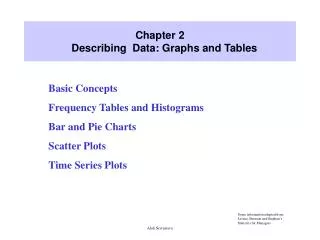
Chapter 2 Describing Data Sets. Chapter 2 Describing Data Sets. 2.1 Introduction 2.2 Frequency Tables and Graphs 2.3 Grouped Data and Histograms 2.4 Stem-and-Leaf Plots 2.5 Sets of Paired Data. Introduction.

Chapter 2 Describing Data Sets
E N D
Presentation Transcript
Chapter 2 Describing Data Sets 2.1 Introduction 2.2 Frequency Tables and Graphs 2.3 Grouped Data and Histograms 2.4 Stem-and-Leaf Plots 2.5 Sets of Paired Data
Introduction • An effective presentation of the data often quickly reveals (顯示) important features such as • their range, • degree of symmetry, • how concentrated (集中) or spread out (分散) they are, • where they are concentrated, and so on. • In this chapter we will be concerned with techniques, both tabular and graphic, for presenting data sets. • Frequency tables and frequency graphs • The histogram • The stem-and-leaf plot • The scatter diagram
Frequency Tables and Graphs • The following data represent the number of days of sick leave (病假)taken by each of 50 workers of a given company over the last 6 weeks: 2, 2, 0, 0, 5, 8, 3, 4, 1, 0, 0, 7, 1, 7, 1, 5, 4, 0, 4, 0, 1, 8, 9, 7, 0, 1, 7, 2, 5, 5, 4, 3, 3, 0, 0, 2, 5, 1, 3, 0, 1, 0, 2, 4, 5, 0, 5, 7, 5, 1 • Frequency tables
Example 2.1 • Use Table 2.1 to answer the following questions: (a) How many workers had at least 1 day of sick leave? (b) How many workers had between 3 and 5 days of sick leave? (c) How many workers had more than 5 days of sick leave? • Solution (a) Since 12 of the 50 workers had no days of sick leave, the answer is 50 −12 = 38. (b) The answer is the sum of the frequencies for values 3, 4, and 5; that is, 4 + 5 + 8 = 17. (c) The answer is the sum of the frequencies for the values 6, 7, 8, and 9. Therefore, the answer is 0 + 5 + 2 + 1 = 8.
Exercise • The following frequency table relates the weekly sales of bicycles at a given store over a 42-week period. (a) In how many weeks were at least 2 bikes sold? (b) In how many weeks were at least 5 bikes sold? (c) In how many weeks were an even number of bikes sold?
Line Graphs, Bar Graphs, and Frequency Polygons • Line graph • Bar graph • Frequency Polygons
Symmetric • A set of data is said to be symmetricabout the value x0 if the frequencies of the values x0 − cand x0 + care the same for all c. • The data set presented in Table 2.2, a frequency table, is symmetric about the value x0=3.
Approximately Symmetric • Data that are “close to” being symmetric are said to be approximately symmetric. • Figure 2.4 presents three bar graphs: • one of a symmetric data set, • one of an approximately symmetric data set, and • one of a data set that exhibits no symmetry.
Exercise • The following table lists all the values but only some of the frequencies for a symmetric data set. Fill in the missing numbers.
Relative Frequency Graphs • If f represents the frequency of occurrence of some data value x, then the relative frequency f/n can be plotted versus x, where n represents the total number of observations in the data set. The relative frequency polygon
Example 2.2 • The 37 winning scores range from a low of 270 to a high of 286. This is the relative frequency table:
Example 2.2 • The following is a relative frequency bar graph of the preceding data.
Pie Charts • A pie chart is often used to plot relative frequencies when the data are nonnumeric. • The data in Table 2.4 give the relative frequencies of types of weapons used in murders in a large midwestern city in 1985.
Grouped Data and Histograms • For some data sets the number of distinct values is too large to utilize. • In such cases, we divide the values into groupings, or class intervals. • The number of class intervals chosen should be a trade-off between (1) choosing too few classes at a cost of losing too much information about the actual data values in a class and (2) choosing too many classes, which will result in the frequencies of each class being too small for a pattern to be discernible(可識別的). • Generally, 5 to 10 class intervals are typical.
Grouped Data • Class boundaries • the endpoints of a class interval • Left-end inclusion convention • a class interval contains its left-end but not its right-end boundary point. • for instance • the class interval 20–30 contains all values that are both greater than or equal to 20 and less than 30
Histograms • Histogram • A bar graph plot of the data, with the bars placed adjacent to each other. • Frequency histogram • The vertical axis of a histogram represents the class frequency. • Relative frequency histogram • The vertical axis of a histogram represents the relative class frequency.
Histograms • Characteristics of data detected by histograms
Histograms • Characteristics of data detected by histograms
Example 2.3 • Table 2.8 gives the birth rates (per 1000 population) in each of the 50 states of the United States. Plot these data in a histogram.
Example 2.3 • Solution • Since the data range from a low value of 12.4to a high of 21.9, let us use class intervals of length 1.5, starting at the value 12. • With these class intervals, we obtain the following frequency table. • A histogram plot of these data is presented as follows.
Example 2.4 • The data of Table 2.9 represent class frequencies for the systolic blood pressure (心臟收縮壓)of two groups of male industrial workers: those aged 30 to 40 and those aged 50 to 60. • We can compute and graph the relative frequencies of each of the classes. This results in Table 2.10.
Example 2.4 • Figure 2.10 graphs the relative frequency polygons for both age groups. • Having both frequency polygons on the same graph makes it easy to compare the two data sets. • For instance, it appears that the blood pressures of the older group are more spread out among larger values than are those of the younger group.
Exercise • The following data set represents the scores on intelligence quotient (IQ) examinations of 40 sixth-grade students at a particular school: 114, 122, 103, 118, 99, 105, 134, 125, 117, 106, 109, 104, 111, 127, 133, 111, 117, 103, 120, 98, 100, 130, 141, 119, 128, 106, 109, 115, 113, 121, 100, 130, 125, 117, 119, 113, 104, 108, 110, 102 (a) Present this data set in a frequency histogram. (b) Which class interval contains the greatest number of data values? (c) Is there a roughly equal number of data in each class interval? (d) Does the histogram appear to be approximately symmetric? Why?
Stem-and-leaf Plots • A stem-and-leaf plot: • A very efficient way of displaying a small-to-moderate size data set. • Such a plot is obtained by dividing each data value into two parts—its stem(莖) and its leaf(葉). • For instance • If the data are all two-digit numbers, then we could let the stem of a data value be the tens digit and the leaf be the ones digit. • That is, the value 84 is expressed as • and the two data values 84 and 87 are expressed (the values should be sorted first)
Example 2.5 • Table 2.11 presents the per capita personal income(平均個人總收入) for each of the 50 states and the District of Columbia (哥倫比亞特區) . • The data are for 2002.
Example 2.5 • The data presented in Table 2.11 are represented in the following stem-and-leaf plot. • Note that the values of the leaves are put in the plot in increasing order.
Example 2.6 • The choice of stems should always be made so that the resultant stem-and-leaf plot is informative about the data. • The following data represent the proportion of public elementary school students that are classified as minority(少數民族) in each of 18cities. 55.2, 47.8, 44.6, 64.2, 61.4, 36.6, 28.2, 57.4, 41.3, 44.6, 55.2, 39.6, 40.9, 52.2, 63.3, 34.5, 30.8, 45.3 • If we let the stem denote the tens digit and the leaf represent the remainder of the value, then the stem-and-leaf plot for the given data is as follows:
Example 2.6 • We could have let the stem denote the integer part and the leaf the decimal part of the value, so that the value 28.2 would be represented as • However, this would have resulted in too many stems (with too few leaves each) to clearly illustrate the data set.
Example 2.7 • The following stem-and-leaf plot represents the weights of 80 attendees (參加者)at a sporting convention(體育大會). • The stem represents the tens digit, and the leaves are the ones digit. • It is clear from this plot that • almost all the data values are between 100 and 200 • the spread is fairly uniformthroughout this region(with the exception of fewer values in the intervalsbetween 100 and 110 and between 190 and 200)
Exercise • The following data represent New York City’s daily revenue (收入)from parking meters (in units of $5000) during 30 days in 2002. 108, 77, 58, 88, 65, 52, 104, 75, 80, 83, 74, 68, 94, 97, 83,71, 78, 83, 90, 79, 84, 81, 68, 57, 59, 32, 75, 93, 100, 88 (a) Represent this data set in a stem-and-leaf plot. (b) Do any of the data values seem “suspicious”(有蹊蹺的)? Why?
Sets of Paired Data • Sometimes a data set consists of pairs of values that have some relationship to each other. • Each member of the data set is thought of as having an xvalue and a yvalue. Intelligence Quotient test
Sets of Paired Data • A scatter diagram: • A useful way of portraying a data set of paired values is to plot the data on a two-dimensional rectangular plot with the xaxis representing thexvalue of the data and the y axis representing theyvalue.
Scatter Diagram • The scatter diagram also appears to have some predictive uses. • For instance, suppose we wanted to predict the salary of a worker whose IQ test score is 120. One way to do this is to “fit by eye” a line to the data set. • A scatter diagram is useful in detecting outliers. • Outliers are data points that do not appear to follow the pattern of the other data points.
Exercise • The following data relate prime lending rates (貸款利率) and the corresponding inflation rate (通貨膨脹率)during 8 years in the 1970s. (a) Draw a scatter diagram. (b) Fit a straight line drawn “by hand” to the data pairs. (c) Using your straight line, predict the prime lending rate in a yearwhose inflation rate is 7.2 percent.
KEY TERMS • Frequency: The number of times that a given value occurs in a data set. • Frequency table: A table that presents, for a given set of data, each distinct data value along with its frequency. • Line graph: A graph of a frequency table. The abscissa specifies a data value, and the frequency of occurrence of that value is indicated by the height of a vertical line. • Bar chart (or bar graph): Similar to a line graph, except now the frequency of a data value is indicated by the height of a bar. • Frequency polygon: A plot of the distinct data values and their frequencies that connects the plotted points by straight lines. • Symmetric data set: A data set is symmetric about a given value x0 if the frequencies of the data values x0 − c and x0 + c are the same for all values of c. • Relative frequency: The frequency of a data value divided by the number of pieces of data in the set. • Pie chart: A chart that indicates relative frequencies by slicing up a circle into distinct sectors.
KEY TERMS • Histogram: A graph in which the data are divided into class intervals, whose frequencies are shown in a bar graph. • Relative frequency histogram: A histogram that plots relative frequencies for each data value in the set. • Stem-and-leaf plot: Similar to a histogram except that the frequency is indicated by stringing together the last digits (the leaves) of the data. • Scatter diagram: A two-dimensional plot of a data set of paired values.