Parameter estimation class 6
Parameter estimation class 6. Multiple View Geometry Comp 290-089 Marc Pollefeys. Content. Background : Projective geometry (2D, 3D), Parameter estimation , Algorithm evaluation. Single View : Camera model, Calibration, Single View Geometry.


Parameter estimation class 6
E N D
Presentation Transcript
Parameter estimationclass 6 Multiple View Geometry Comp 290-089 Marc Pollefeys
Content • Background: Projective geometry (2D, 3D), Parameter estimation, Algorithm evaluation. • Single View: Camera model, Calibration, Single View Geometry. • Two Views: Epipolar Geometry, 3D reconstruction, Computing F, Computing structure, Plane and homographies. • Three Views: Trifocal Tensor, Computing T. • More Views: N-Linearities, Multiple view reconstruction, Bundle adjustment, auto-calibration, Dynamic SfM, Cheirality, Duality
Parameter estimation • 2D homography Given a set of (xi,xi’), compute H (xi’=Hxi) • 3D to 2D camera projection Given a set of (Xi,xi), compute P (xi=PXi) • Fundamental matrix Given a set of (xi,xi’), compute F (xi’TFxi=0) • Trifocal tensor Given a set of (xi,xi’,xi”), compute T
DLT algorithm • Objective • Given n≥4 2D to 2D point correspondences {xi↔xi’}, determine the 2D homography matrix H such that xi’=Hxi • Algorithm • For each correspondence xi ↔xi’ compute Ai. Usually only two first rows needed. • Assemble n 2x9 matrices Ai into a single 2nx9 matrix A • Obtain SVD of A. Solution for h is last column of V • Determine H from h
measured coordinates estimated coordinates true coordinates Error in one image Symmetric transfer error Geometric distance d(.,.) Euclidean distance (in image) e.g. calibration pattern Reprojection error
Analog to conic fitting Geometric interpretation of reprojection error Estimating homography~fit surface to points X=(x,y,x’,y’)T in 4
Maximum Likelihood Estimate Statistical cost function and Maximum Likelihood Estimation • Optimal cost function related to noise model • Assume zero-mean isotropic Gaussian noise (assume outliers removed) Error in one image
Maximum Likelihood Estimate Statistical cost function and Maximum Likelihood Estimation • Optimal cost function related to noise model • Assume zero-mean isotropic Gaussian noise (assume outliers removed) Error in both images
Error in two images (independent) Varying covariances Mahalanobis distance • General Gaussian case Measurement X with covariance matrix Σ
Invariance to transforms ? will result change? for which algorithms? for which transformations?
Non-invariance of DLT Given and H computed by DLT, and Does the DLT algorithm applied to yield ?
for similarities Effect of change of coordinates on algebraic error so
Non-invariance of DLT Given and H computed by DLT, and Does the DLT algorithm applied to yield ?
Invariance of geometric error Given and H, and Assume T’ is a similarity transformations
Or Normalizing transformations • Since DLT is not invariant, what is a good choice of coordinates? e.g. • Translate centroid to origin • Scale to a average distance to the origin • Independently on both images
Importance of normalization 1 ~104 ~102 ~102 ~102 ~102 ~102 1 ~104 orders of magnitude difference!
Normalized DLT algorithm • Objective • Given n≥4 2D to 2D point correspondences {xi↔xi’}, determine the 2D homography matrix H such that xi’=Hxi • Algorithm • Normalize points • Apply DLT algorithm to • Denormalize solution
Iterative minimization metods Required to minimize geometric error • Often slower than DLT • Require initialization • No guaranteed convergence, local minima • Stopping criterion required Therefore, careful implementation required: • Cost function • Parameterization (minimal or not) • Cost function ( parameters ) • Initialization • Iterations
Parameterization Parameters should cover complete space and allow efficient estimation of cost • Minimal or over-parameterized? e.g. 8 or 9 (minimal often more complex, also cost surface) (good algorithms can deal with over-parameterization) (sometimes also local parameterization) • Parametrization can also be used to restrict transformation to particular class, e.g. affine
Function specifications • Measurement vector XNwith covariance Σ • Set of parameters represented by vector P N • Mapping f: M →N. Range of mapping is surface S representing allowable measurements • Cost function: squared Mahalanobis distance Goal is to achieve , or get as close as possible in terms of Mahalanobis distance
Symmetric transfer error Error in one image Reprojection error
Initialization • Typically, use linear solution • If outliers, use robust algorithm • Alternative, sample parameter space
Iteration methods Many algorithms exist • Newton’s method • Levenberg-Marquardt • Powell’s method • Simplex method
Gold Standard algorithm • Objective • Given n≥4 2D to 2D point correspondences {xi↔xi’}, determine the Maximum Likelyhood Estimation of H • (this also implies computing optimal xi’=Hxi) • Algorithm • Initialization: compute an initial estimate using normalized DLT or RANSAC • Geometric minimization of -Either Sampson error: • ● Minimize the Sampson error • ● Minimize using Levenberg-Marquardt over 9 entries of h • or Gold Standard error: • ● compute initial estimate for optimal {xi} • ● minimize cost over {H,x1,x2,…,xn} • ● if many points, use sparse method
Robust estimation • What if set of matches contains gross outliers?
RANSAC • Objective • Robust fit of model to data set S which contains outliers • Algorithm • Randomly select a sample of s data points from S and instantiate the model from this subset. • Determine the set of data points Si which are within a distance threshold t of the model. The set Si is the consensus set of samples and defines the inliers of S. • If the subset of Si is greater than some threshold T, re-estimate the model using all the points in Si and terminate • If the size of Si is less than T, select a new subset and repeat the above. • After N trials the largest consensus set Si is selected, and the model is re-estimated using all the points in the subset Si
Distance threshold Choose t so probability for inlier is α (e.g. 0.95) • Often empirically • Zero-mean Gaussian noise σ then follows distribution with m=codimension of model (dimension+codimension=dimension space)
How many samples? Choose N so that, with probability p, at least one random sample is free from outliers. e.g. p=0.99
Acceptable consensus set? • Typically, terminate when inlier ratio reaches expected ratio of inliers
Adaptively determining the number of samples e is often unknown a priori, so pick worst case, e.g. 50%, and adapt if more inliers are found, e.g. 80% would yield e=0.2 • N=∞, sample_count =0 • While N >sample_count repeat • Choose a sample and count the number of inliers • Set e=1-(number of inliers)/(total number of points) • Recompute N from e • Increment the sample_count by 1 • Terminate
Robust Maximum Likelyhood Estimation Previous MLE algorithm considers fixed set of inliers Better, robust cost function (reclassifies)
Other robust algorithms • RANSAC maximizes number of inliers • LMedS minimizes median error • Not recommended: case deletion, iterative least-squares, etc.
Automatic computation of H • Objective • Compute homography between two images • Algorithm • Interest points: Compute interest points in each image • Putative correspondences: Compute a set of interest point matches based on some similarity measure • RANSAC robust estimation: Repeat for N samples • (a) Select 4 correspondences and compute H • (b) Calculate the distance d for each putative match • (c) Compute the number of inliers consistent with H (d<t) • Choose H with most inliers • Optimal estimation: re-estimate H from all inliers by minimizing ML cost function with Levenberg-Marquardt • Guided matching: Determine more matches using prediction by computed H • Optionally iterate last two steps until convergence
Determine putative correspondences • Compare interest points Similarity measure: • SAD, SSD, ZNCC on small neighborhood • If motion is limited, only consider interest points with similar coordinates • More advanced approaches exist, based on invariance…
Example: robust computation Interest points (500/image) Putative correspondences (268) Outliers (117) Inliers (151) Final inliers (262)
Assignment • Take two or more photographs taken from a single viewpoint • Compute panorama • Use different measures DLT, MLE • Use Matlab • Due Feb. 13
Next class: Algorithm evaluation and error analysis • Bounds on performance • Covariance propagation • Monte Carlo covariance estimation