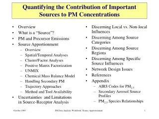
Quantifying the Contribution of Important Sources to PM Concentrations

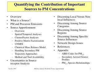
1. Quantifying the Contribution of Important Sources to PM Concentrations • Overview • What is a Source? • Emissions • Source Attribution Methods and Tools • Discerning Among Source Categories • Discerning Among Source Regions • Discerning Among Specific Source Influences • Uncertainties in Source-receptor Analyses • Network Design Issues • References/Appendix with PM2.5 AIRS codes PM Data Analysis Workbook: Source Attribution

2. Overview • Why do we need to understand the sources of PM? When an area experiences elevated concentrations of PM, particularly when the concentrations are in exceedance of the standard, research and analysis is needed to investigate the possible sources of PM and PM precursors leading to the high concentrations. The analysis and research required spans all aspects of the regulatory community: • Monitoring staff need to know whether or not their sampling and analysis set up is adequate to identify the PM and precursor species that are critical for identifying potential sources in their area. • Analysts need to be able to identify potential sources and meteorological conditions to assist policy makers and modelers in developing control strategies. • Modelers need to know how well current emission inventories and dispersion models represent the ambient conditions so that they can model future control scenarios and the effect on PM concentrations. • Policy makers need to know what sources are the principal contributors to PM so that appropriate controls on PM and precursor emissions can be developed and implemented. • In a previous chapter of the workbook, data analyses exploring the spatial and temporal characteristics of PM data were discussed. In this chapter, we first discuss “what is a source?”. Important emissions sources are then described as well as source attribution methods and tools and their uncertainties. Examples are then provided of how to discern among source categories, source regions, and specific source influences. PM Data Analysis Workbook: Source Attribution

3. What is a “Source”?: Primary versus Secondary • Primary PM are composed of material in the same chemical form as when they were emitted to the atmosphere including windblown dust, sea salt, road dust, mechanically generated particles and combustion-generated particles such as fly ash and soot. This also includes particles formed from the condensation of high temperature vapors formed during combustion (e.g., As, Se, Zn). Concentrations of primary PM are a function of emission rate, transport and dispersion, and removal rate. • Secondary particles are formed from condensable vapors generated by chemical reactions of gas-phase precursors. Secondary processes can result in either the formation of new particles or the addition of PM to preexisting particles. For example, sulfate in PM is mostly formed by atmospheric oxidation of SO2. Also, oxides of nitrogen react in the atmosphere to form nitric acid vapor which in turn may react with NH3 to form particulate ammonium nitrate. A portion of the organic aerosol is also due to secondary processes. Secondary formation is a function of many factors including: concentrations of precursors, concentrations of other gaseous reactive species (e.g., ozone, hydroxyl radical), atmospheric conditions, and cloud or fog droplet interactions. It is considerably more difficult to relate ambient concentrations of secondary species to sources of precursor emissions than it is to identify the sources of primary particles. PM Data Analysis Workbook: Source Attribution

4. What is a “Source”?: Local vs. Transport • A key question analysts face is “how do I tell the difference between locally generated PM and PM transported into the area?” Policy makers need to understand how much of the PM problem is under their jurisdiction to control. • Techniques for assessing the difference between local and transported PM include: • Spatial and temporal analyses (e.g., Are high concentrations observed on a regional basis or only at a few “hot spots”?) • Assessing the age of an air mass accompanied with trajectory analysis • The use of “tracers-of opportunity” and species ratios accompanied with trajectory analysis (e.g., using potassium to identify forest fire impact) • The use of satellite information to corroborate transport (e.g., Saharan dust storm impact on United States sites) PM Data Analysis Workbook: Source Attribution

5. What is a “Source”?: Other Issues • Regional issues. Analysts need to be able to assess how much an urban area is contributing to a PM exceedance problem compared to the regional background. • As a first approximation of local versus regional contributions to an urban area’s PM, the differences between the concentrations of average urban and nearby rural monitoring data could be assessed. This assumes that the PM at the rural sites are not “contaminated” by the urban emissions and that the same regional sources have the same impact on the rural monitors as the urban monitors (see Schichtel, 1999). • Another approach is to model the PM dependence on wind speed and wind direction to classify a site as being dominated by local or regional source contributions (Schichtel, 1999). • Researchers are investigating the development of “regional background” profiles to assist in apportioning PM. These profiles could be used in an attempt to quantify the regional contribution to PM concentrations. • Studies have shown that samplers were strongly influenced by sources less than 10 km away and that even minor sources close to the sampler could overwhelm any regional component in a 24-hr integrated sample (VanCuren, 1998). Others have shown that individual emitters have a zone of influence less than 1 km (e.g., Chow et al., 1999). PM Data Analysis Workbook: Source Attribution

6. PM Emissions • Knowledge of PM emissions is required for performing source apportionment and assessing control measures. • The majority of the PM2.5 mass over the US is of secondary origin, formed within the atmosphere through gas-particle conversion of precursor gases such as sulfur oxides, nitrogen oxides, and organics. • Precursor emissions that are well defined include sulfur (SO2) and nitrogen (NOx) while the emissions of other species such as organics, soil, and soot are poorly defined. Key citation: Schichtel (1999) PM Data Analysis Workbook: Source Attribution

7. North American SO2 Emission Rates The highest SO2 emission rates occur over the Ohio River Valley, eastern seaboard, and urban locations, such as Atlanta and St. Louis. There are few major SO2 sources in the west. PM Data Analysis Workbook: Source Attribution

8. North American NOx Emission Rates • Area source NOx emissions are highest near cities. • Point source emissions are highest over the Industrial Midwest. PM Data Analysis Workbook: Source Attribution

9. Meat-cooking operations Paved road dust Fireplaces Noncatalyst gasoline vehicles Diesel vehicles Surface Coating Forest Fires Cigarettes Catalyst-equipped gasoline vehicles Organic chemical processes Brake lining Roofing tar pots Tire wear Misc. industrial point sources Natural gas combustion Misc. petroleum industry processes Primary metallurgical processes Railroad (diesel oil) Residual oil stationary sources Refinery gas combustion Major Sources of OC Emissions Adapted from Cass, 1997 Sources listed most abundant to least abundant for the Los Angeles urban area for 1982. PM Data Analysis Workbook: Source Attribution

10. Emissions Issues • PM2.5 precursor emissions patterns vary across the US; thus, PM2.5 speciation and concentrations also vary. • Of importance to source apportionment is guidance on the following: • validating emission profiles and inventories • improving emission profiles and inventories • estimating emission profiles and inventories • identifying unusual events • Many of these topics are covered in the introduction and in the emission inventory evaluation sections of the workbook. PM Data Analysis Workbook: Source Attribution

11. Source Apportionment Overview (1 of 3) • Relating source emissions to their quantitative impact on ambient air pollution is referred to as source apportionment. In principle source apportionment can be performed in two complementary ways. The traditional approach is dispersion modeling, in which a pollutant emission rate and meteorological information are input to a mathematical model that disperses (and may also chemically transform) the emitted pollutant, generating a prediction of the resulting pollutant concentration at a point in space and time. The inputs may be measured quantities but they need not be, in which case the modeling is a "what if" exercise which explores the consequences of different emission rate and meteorological variable possibilities. The alternative is receptor modeling, which may be defined as "a specified mathematical procedure for identifying and quantifying the sources of ambient air contaminants at a receptor primarily on the basis of concentration measurements at that receptor." The concentration measurements referred to are those of particular chemical or physical properties that are characteristic of particular source emissions. In contrast to dispersion modeling, receptor modeling is diagnostic, not prognostic - it describes the past rather than the future. In further contrast to dispersion modeling, receptor modeling has everything to do with measurements and cannot be performed without them. While source apportionment in principle embraces both modeling approaches, in common usage it is often taken as synonymous with receptor modeling. This overview is concerned only with this restricted meaning of source apportionment. • Two milestones in the development of receptor modeling are worth noting. First, the Friedlander (1973) article is generally recognized as the genesis of the chemical mass balance (CMB) receptor model, referred to at the time as chemical element balance. CMB has a special status in the receptor modeling toolbox, being the only model up to the present that has been officially approved (i.e., supported and distributed) by EPA. CMB is described elsewhere in this document. • A second milestone was the 1982 Mathematical and Empirical Receptor Models Workshop, now known as "Quail Roost II", and the series of articles that resulted from it. The workshop was important for multiple reasons: (a) It introduced the concept of sophisticated synthetic (simulated) data sets as test beds for comparing the performance of alternative receptor modeling approaches, where the "truth" is known a priori by the constructors of the data sets; (b) it brought together many of the U.S. receptor modeling practitioners in a "blind" intercomparison of their various methods when applied to common data sets, including both synthetic and real sets; and (c) it resulted in a Glossary of receptor modeling terms that provided a common language for this emerging field. The degree of success that was achieved in (b) was instrumental in bringing EPA to a realization of the potential importance of receptor modeling as a complement to traditional dispersion modeling for source apportionment. PM Data Analysis Workbook: Source Attribution

12. Source Apportionment Overview (2 of 3) • Receptor model types may be classified as single-sample or multivariate. In the first type the modeling analysis is performed independently on each available sample. The simplest example of this is the 'tracer element' method, in which a particular property (e.g., chemical specie) is known to be uniquely associated with a specific source, so that the total ambient mass impact of the source may be estimated by dividing the measured ambient concentration of the property by the property's known abundance in the source's emissions. The method is not often available because of the difficulties of finding unique tracers or knowing their abundances. However even if the property is not uniquely associated with a source of interest, if its abundance in that source is known, then the method can always be used to provide an upper limit for the source's impact. A novel example of this method is the use of the radiocarbon (14C) content of an ambient sample to estimate the fraction of carbon in the sample that is biogenic (non-fossil-fuel related). • The best-known example of single-sample receptor modeling is of course chemical mass balance. CMB removes the need for unique tracers of sources, but still requires the abundances of the chemical components of each source (source profiles) to be known. • Multivariate receptor models require the input of data from multiple samples, and extract the source apportionment information from all of the sample data simultaneously. The reward for the extra complexity of these models is that they purport to estimate not only the source contributions but the source compositions (profiles) as well. The simplest example of a multivariate method is 'tracer element/multiple linear regression'. This method requires tracers that are uniquely associated with the sources of interest, but does not require their abundances to be known. • Additional multivariate receptor models include (a) absolute principal component analysis, (b) specific rotation factor analysis, (c) target transformation factor analysis, (d) three-mode factor analysis, (e) source profiles by unique ratios - SPUR, (f) receptor model applied to patterns in space - RMAPS, (g) UNMIX, and (h) positive matrix factorization. Most of these models are based on factor analysis, or the closely related principal component analysis. In recent years the development and investigation of the last three has been supported by EPA. In comparison with CMB far less is understood about the behavior and validity of these multivariate models. Criticisms have been directed at specific models, in addition to the general criticism of any factor analysis-based model that does not employ additional constraints to limit the solution space. PM Data Analysis Workbook: Source Attribution

13. Source Apportionment Overview (3 of 3) • One of the challenges that receptor modeling will need to confront in the PM2.5 arena is the treatment of secondary mass - products that result from atmospheric transformation processes between source and receptor, such as sulfate and nitrate. While this has always been a problem for receptor modeling, it is more severe for PM2.5 than for PM10 because the secondary contribution to PM2.5 is a larger fraction than for PM-10. CMB deals with this in a limited way that isolates the total mass of a secondary component (e.g., sulfate) but cannot apportion it to individual sources. Progress in this area will require a hybrid receptor model approach, i.e., the use of selected emissions rate, meteorological, and chemical transformation information with an otherwise conventional receptor model. Receptor modeling was invented for the very reason of avoiding the need for such frequently uncertain information, but it seems inevitable that source apportionment of secondaries will require an extension of classical receptor modeling. By combining elements of both receptor and dispersion models the intent is to minimize the weaknesses of the separate approaches and maximize their combined strengths. • The development of receptor modeling over the past two decades has been strongly influenced by the extensive use of inorganic species, particularly atomic elements measured by x-ray fluorescence. In the receptor modeling of PM2.5 there is likely to be a new emphasis on organic species. This is because of the relatively greater contribution of combustion sources and carbon to PM2.5 than to PM10. This will not be an easy transition, because of formidable difficulties in organic aerosol sampling (both positive and negative artifacts can occur) and analysis (the presence of a bewildering number of organic species, frequently at low concentrations). The Northern Front Range Air Quality Study recently performed in the Denver area, and the continuing characterization of organic aerosol in Southern California, provide some indications of the promise of this new direction. Key citation: Lewis, 1999 PM Data Analysis Workbook: Source Attribution

14. Source Attribution Methods and Tools • Source attribution methods are used to resolve the composition of PM into components related to emission sources. Several methods are available. • It is useful to apply more than one method (since data requirements differ among them) and look for consensus among results. • Methods and tools discussed in this section include the following: • Spatial and temporal characteristics of data • Cluster, factor, and other multivariate statistical techniques • PMF • UNMIX • Source-receptor models: CMB8 PM Data Analysis Workbook: Source Attribution

15. Using Spatial and Temporal Data • Potassium nitrate is a major component of all fireworks. • This figure shows all available PM2.5 K data from all N. American sites, averaged to produce a continental average for each day during 1988-1997. • Fourth of July celebration fireworks are clearly observed in the potassium time series. • Fireworks displays on local holidays/events could have a similar affect on data. Poirot (1998) Regional averaging and count of sample numbers were conducted in Voyager, using variations of the Voyager script on p. 6 of the Voyager Workbook Kvoy.wkb. Additional averaging and plotting was conducted in Microsoft Excel. PM Data Analysis Workbook: Source Attribution

16. Spatial and Temporal Analyses • A simple material balance on the annual average chemical composition can be useful (shown here: Los Angeles area PM2.5). • EC concentrations were highest in Central LA, consistent with fresh motor vehicle emissions and traffic density. • OC concentrations typically accounted for the largest portion of the PM2.5 at most sites. More emphasis on OC measurements may be warranted. • Nitrate and ammonium concentrations were highest at the downwind site (Rubidoux) consistent with NH3 emission sources and secondary nitrate formation. Made using Excel; adapted from Cass, 1997. Sites are arranged from west to east (the general direction of transport in the Los Angeles basin. PM Data Analysis Workbook: Source Attribution

17. Simple analyses of wind direction and PM species concentrations can be used to begin an assessment of likely sources. Temporal resolution less than 24-hr of the PM data may be necessary for this analysis. PM10 zinc concentrations at Crows Landing with respect to wind direction are shown. High concentrations in the northwest sector are consistent with the refuse incinerator located one km to the NNW of the monitoring site. Spatial and Temporal Analyses Zinc concentration distribution with respect to wind direction (%) Adapted from wind roses reported by Chow et al., 1996. Radar plot prepared in Excel. Wind direction is the direction from which the wind is blowing. Data from Crows Landing, CA during 1990 summer intensive study. PM Data Analysis Workbook: Source Attribution

18. Multivariate Analyses • Multivariate analyses are statistical procedures used to infer the mix of hydrocarbon sources impacting a receptor location. • Procedures including cluster, factor/principal component, regression, and other multivariate techniques are usually available in statistical software packages. • Literature review shows many refinements and options to these analyses. • A drawback to these analyses is that the analyst must infer how certain statistical species groupings relate to emissions sources. • A nice feature of these analyses is the ability to summarize a multivariate data set using a few components. PM Data Analysis Workbook: Source Attribution

19. Key PM Species and Sources (1 of 3) PM Data Analysis Workbook: Source Attribution

20. Key PM Species and Sources (2 of 3) PM Data Analysis Workbook: Source Attribution

21. Key PM Species and Sources (3 of 3) PM Data Analysis Workbook: Source Attribution

22. Cluster and Factor Analyses • Cluster analysis is a multivariate procedure for detecting natural groupings in data. • To produce clusters, you must be able to compute some measure of dissimilarity between objects. • Correlation measures are often used because they are not influenced by differences in scale between objects. This is important because PM species concentrations can vary over several orders of magnitude. • Factor analysis is a method of decomposing a correlation or covariance matrix. • Factors indicate the best associations among variables while regression lines indicate the best predictions. • The factor model expresses the variation within and the relations among observed variables as partly common variation among factors and partly specific variation among random errors. PM Data Analysis Workbook: Source Attribution

23. Cluster/Factor Analysis Example Example PM2.5 cluster and factor analyses to be developed PM Data Analysis Workbook: Source Attribution

24. PMF Description • Positive matrix factorization (PMF) can be used to determine source profiles based on the ambient data. • The major difference between principal component analysis and PMF is that only positive factors can be generated with PMF (no negative concentrations). • Also PMF does not rely on information from the correlation matrix but uses a point-by-point least-squares minimization scheme. Profiles produced using PMF can be directly compared to the input matrix since the profiles are in the same units as the input data. PM Data Analysis Workbook: Source Attribution

25. PMF Analysis Example (1 of 2) • Polissar et al. (1998) used PMF to investigate the fine particle composition data from seven National Park Service locations in Alaska for the period 1986-1995. The sites included the Northwest Alaska Areas National Park (NWAA), Bering Land Bridge National Preserve (BELA), Gates of the Arctic National Park (GAAR), Denali National Park (DENA), Yukon Charley National Preserve (YUCH), Wrangell St. Elias National Park (WRST), and Katmai National Park (KATM). • PMF uses the estimates of the error in the data to provide optimum data point scaling and permits a better treatment of missing and below detection limit values. • Up to eight source components were obtained for the data sets: PM Data Analysis Workbook: Source Attribution

26. PMF Analysis Example (2 of 2) • The highest average PM2.5 concentration at the Bering Land Bridge site (BELA) may be due to the strong influence of aerosol emissions from local pollution sources in nearby Nome plus PM transported into the region. • Note the large seasonal difference in the forest fire factor at Gates of the Arctic (GAAR). Polissan et al., 1998 PM Data Analysis Workbook: Source Attribution

27. UNMIX • UNMIX is a multivariate receptor modeling package that inputs observations of particulate composition and seeks to find the number, composition, and contributions of the contributing sources or source types. UNMIX also produces estimates of the uncertainties in the source compositions. UNMIX uses a generalization of the self-modeling curve resolution method developed in the chemometrics community (Henry, 1997). • Data Requirements: UNMIX inputs data in tabular format as flat ASCII files. Each column represents one species and each row is one sample or observation. It is very helpful to have a measure of total mass included in the data. It is generally best to analyze data from one site at a time. Basically, the more data the better, in terms of both species and observations. The upper limit on the amount of data is determined by the size of the computer. Based on experience, the practical lower limit on the number of observations is 50 to 100. • System Requirements: UNMIX is currently implemented as a MATLAB program(see the website mathworks.com for more information). UNMIX has a graphical user interface so the user need not be familiar with MATLAB itself. PM Data Analysis Workbook: Source Attribution

28. UNMIX Analysis Example Example PM2.5 UNMIX analyses to be developed PM Data Analysis Workbook: Source Attribution

29. Chemical Mass Balance Modeling • The purpose of CMB receptor modeling is to apportion ambient PM to emission sources. The source apportionment of ambient PM provides independent evaluation of the relative contributions of sources to ambient levels of PM. • The CMB model uses an effective variance least squares solution to a set of linear equations which express each measured chemical species concentration as a linear sum of products of source profile species and source contributions. • Model input includes: • Source profile species (fractional amount of species in the PM emissions from each source type). • Receptor (ambient) concentrations. • Realistic uncertainties for source and receptor values. Input uncertainty is used to weigh the relative importance of input data to model solutions and to estimate uncertainty of the source contributions. • Model output includes: • Contributions from each source type to the total ambient VOC and individual hydrocarbon species and the uncertainty. • Performance parameters. PM Data Analysis Workbook: Source Attribution

30. CMB Model Assumptions CMB model assumptions include the following: • Composition of source emissions are constant over the ambient and source sampling period (can tolerate substantial variabilities). • Chemical species do not react with each other (i.e., they add linearly) (little known about this). • All sources which may significantly contribute to the receptor have been identified and their emissions characterized (minor contributors may be omitted). • Number of source categories £ number of chemical species (the larger the difference, the better). • Source profiles are linearly independent (degree of independence depends on the variability of the source profile). • Measurement errors are random, uncorrelated, and normally distributed (effects unknown). PM Data Analysis Workbook: Source Attribution

31. CMB Application Protocol (1 of 2) • Assessmodel applicability (e.g., data from well-characterized methods, large number of species, major sources identified, source profiles available, and reasonable uncertainties attached). • Selectsource profiles for potential contributors (e.g., area, natural, and point sources plus other sources identified in preliminary analyses). • Select sources for inclusion in the CMB solution (e.g., upwind point, seasonal emitters, non-collinear profiles). • Determine initial source contribution estimates (SCE) (e.g., use variety of source profiles and fitting species combinations, determine effects on results of alternate source profiles). May need to combine similar source types due to collinearity. • Examine model outputs and performance measures. Do spatial and temporal results make sense considering meteorology and source emission patterns? PM Data Analysis Workbook: Source Attribution

32. CMB Application Protocol (2 of 2) • Check how the removal and addition of some species affects results. The source profiles need to be the most precise for the most influential species. • Identifydeviations from model assumptions (e.g., source compositions constant, all sources included, source profiles independent, etc.). • Identify and correct model input errors (e.g., increase uncertainty of profiles, provide different composites, identify and characterize missing sources, stratify samples by meteorology). • Verify consistency and stability of SCE (substitute different profiles for same source type, add or drop species form fit, examine source contributions to individual species). • Evaluate results of CMB with respect to other source assessment methods (e.g., compare SCEs among nearby sites, compare source contribution variations over time with expected emissions and meteorology, apply other receptor methods and compare results, apply dispersion models and compare results). PM Data Analysis Workbook: Source Attribution

33. CMB Performance Goals (1 of 2) • Chi square (2) is used to consider the uncertainty of the calculated species concentrations (weighted sum of squares of the differences between calculated and measured fitting species concentrations). Values < 1.0 indicate a very good fit. • The percent mass is the percent ratio of the sum of model-calculated SCEs to the measured mass concentration. This is used to track the percent explained mass; a value near 100 percent can be misleading because poor fits can force a high percent mass. • The t-statistic is the ratio of the SCE to its standard error. The standard error of the SCE is an indicator of the precision in the model estimates. Values < 2.0 identify model estimates that are not significantly different from 0. • Degrees of freedom is the number of species in the fit minus the number of sources in the fit. • R2 is used to measure the variance in the ambient species concentrations, which is explained by the calculated species concentrations via linear regression. The closer the value is to 1.0, the better the SCEs explain the measured concentrations. • Standard error is the variance of the SCE. PM Data Analysis Workbook: Source Attribution

34. CMB Performance Goals (2 of 2) • The ratio of the calculated species mass (CALC) to measured species mass (MEAS) is used to identify species that are over- or under-accounted for by the model. A ratio >1.0 means that more mass for a given species was accounted for by the model than was measured in the ambient sample. • The ratio of the residuals to the uncertainty is the signed difference between CALC and MEAS divided by the uncertainty of the difference. It is used to identify species that are over- and under-accounted for by the model. • The normalized modified pseudo-inverse matrix (MPIN), a diagnostic output of CMB7, indicates the degree of influence each species concentration has on the contribution and standard error of the corresponding source category. MPIN is normalized such that it takes on values from -1.0 to 1.0. Species with MPIN absolute values of 1.0 to 0.5 are associated with influential species. • Maximum source uncertainty and minimum source projection (Henry, 1992) are used to assess clusters of sources which the model cannot easily distinguish between and that are likely to be interfering with the model's ability to provide a good set of SCEs. PM Data Analysis Workbook: Source Attribution

35. Source Profiles • Use profiles that are representative of the study area during the period when ambient data were collected. • Include ubiquitous sources such as gasoline and diesel exhaust, secondary components (sulfate, nitrate, ammonium), sea salt (if coastal site), vegetative burning (e.g., forest fires, residential fireplaces), and crustal material. • Include point sources identified in the emission inventory. • Try available source profiles in sensitivity tests to determine the best ones for use (minimize collinearity). PM Data Analysis Workbook: Source Attribution

36. How to Obtain Source Profiles Source profiles may be obtained from the following sources: • Source measurements made in your region during the period for which ambient data are available. See http://charon.cira.colostate.edu/DRIFinal/ for Northern Front Range air quality study source profiles. • Literature review. Key references are included in the reference section. • EPA SPECIATE (http://www.epa.gov/ttn/chief/software.html#speciate) • Analysis of ambient data using tools such as PMF and UNMIX. PM Data Analysis Workbook: Source Attribution

37. CMB Example Analyses (1 of 2) Seattle area, Washington • Note seasonal differences in monthly average PM2.5 source contribution percentages of burning (fall/winter) and secondary sulfate (summer). • Differences in winter and summer burning contributions are also noticeable using pie charts for the data set. From Maykut et al. Prepared with Excel PM Data Analysis Workbook: Source Attribution

38. CMB Example Analyses (2 of 2) • When additional organic carbon species and source profiles are available, CMB can be used to provide substantial breakdown of the organic carbon component. • The dominant sources of PM2.5 organic aerosol were diesel exhaust, gasoline exhaust, meat cooking, and woodsmoke. Made using Excel; adapted from Cass, 1997 Other organics include paved road dust, cigarette smoke, vegetative detritus, tire wear debris, and secondary organics. PM Data Analysis Workbook: Source Attribution

39. Checking Source Apportionment Results • Three Kraft paper mills in the Washington state study area are located to the south, north, and northwest of the monitoring site. • Agreement between the wind directions associated with specific profiles and the actual locations of the sources adds credibility to the source apportionment results. From Maykut et al. Plot: nanograms of PM attributed to the source by wind direction. PM Data Analysis Workbook: Source Attribution

40. Method and Tool Availability • Species relationships and the development of reasonable constraints on the data can be investigated using scatter plots. • Cluster, factor, and principal component analyses and linear regression are available in most standard statistical packages. • A beta version of PMF is currently being tested by EPA. • A beta version of UNMIX is being tested by EPA and others. Contact Ron Henry for a copy (rhenry@usc.edu) • CMB8 modifications are planned. The current version is available from ftp://eafs.sage.dri.edu/cmb80/model/ PM Data Analysis Workbook: Source Attribution

41. Uncertainties in Source-Receptor Analyses • Many emitters have similar species composition profiles. The practical implication of this limitation is that one may not be able to discern between the dust emitted by agricultural practices and dust emitted by mobile sources on unpaved roads. • Species composition profiles change between source and receptor. Most source-receptor models cannot currently account for changes due to photochemistry. Since nitrates, sulfates, and some organic carbon compounds are primarily of secondary origin, current methods cannot tie these compounds to their primary emission sources. • Receptor models cannot predict the consequences of emissions reductions. One cannot estimate source profiles resulting from changes in emissions and predict ambient concentrations using receptor models. PM Data Analysis Workbook: Source Attribution

42. Discerning Local vs. Non-local Influences • Background and Rationale • Influence of wind speed on local concentrations • Mid-Atlantic Rural Sites PM2.5 vs. Surface Wind Speed • Mid-Atlantic Urban Sites PM2.5 vs. Surface Wind Speed • Seasonal Urban-Rural Difference • Conclusions Key citation: Schichtel (1999) PM Data Analysis Workbook: Source Attribution

43. Background and Rationale • At any given location, the PM concentration is the combination of the PM mass originating from non-local sources transported in and the PM mass originating from local sources. • The local/non-local contributions depend on emissions, transport and aerosol formation and removal processes, so there is no “typical” non-local concentration. • Quantifying the local contributions identifies the part of the PM problem that can be controlled locally. PM Data Analysis Workbook: Source Attribution

44. Influence of Wind Speed on Local Concentrations • The concentration C is equal to the sum of the background (Co) and local contribution (QL/UH) • Assuming a fixed source region length (L), emission rate (Q) and mixing height (H), as the wind speed (U) increases the concentration from the local sources decreases asymptotically approaching the background concentration. PM Data Analysis Workbook: Source Attribution

45. PM2.5 vs. Surface Wind Speed at Urban and Rural Sites The PM2.5 at these urban sites during the cold season (Nov - March) decline sharply (60%) with increasing wind speeds compared to the rural sites (30%). This implies the urban PM2.5 is dominated by local sources. PM Data Analysis Workbook: Source Attribution

46. Local Emission Influenced PM2.5 • Local PM emissions cause concentrations at sites 9, 10, & 11 to have a different temporal pattern with higher concentrations than the other, more regional sites • Concentrations at sites 9, 10, & 11 are above 35 μg/m3 on September 15, 1994 but concentrations decrease to less than 30 μg/m3 within three kilometers. PM Data Analysis Workbook: Source Attribution

47. Seasonal Urban-Rural Difference • The excess PM2.5 at Washington DC ranges from >10 mg/m3 in the winter to 1-2 mg/m3 in the summer. • The Phoenix excess PM2.5 ranges from 11 - 16 mg/m3 in the winter to 3 mg/m3 in the summer. PM Data Analysis Workbook: Source Attribution

48. Local vs. Non-local Sources: Conclusions • In the examples shown here using IMPROVE data, Mid-Atlantic and Southwest urban center PM2.5 concentrations are dominated by local sources during the winter. Concentrations and wind speed were used to assess this. • At the Mid-Atlantic urban sites, the summer local sources contribute about 10% of the PM mass compared to up to 70% in the winter. • At the urban Southwest, the local sources contribute about 30% of the summertime PM mass compared to about 80% in the winter. • Careful comparison of urban and rural site data in a region, with the use of meteorological data, can be used to assess local vs. non-local contributions to PM. PM Data Analysis Workbook: Source Attribution

49. Discerning Among Source Categories • Natural vs. anthropogenic sources • Anthropogenic source categories • Wood smoke • Utilities • Motor vehicles • Refinement of anthropogenic source categories • Dust from anthropogenic activities: soil types and sources • Proscribed burn vs. wood stoves • Oil vs. coal utilities • Motor vehicle exhaust vs. evaporative vs. diesel, etc. PM Data Analysis Workbook: Source Attribution

50. Using Spatial and Temporal Analyses Concentrations of PM2.5 iron with silicon, aluminum, and potassium at Chiricahua National Park in Arizona. • Fe and Al concentrations strongly correlate, suggesting a common source influence. Ratios are consistent with soil. • Fe and K concentrations do not correlate as well. The lower K:Fe ratio of 0.6 is indicative of soil. Higher ratios are consistent with woodsmoke. • Data corresponding to the July 4th weekend are highlighted. Poirot, (1998) Microsoft Excel used to prepare scatter plot and calculate regression coefficients. PM Data Analysis Workbook: Source Attribution