Dorf and Bishop, Modern Control Systems

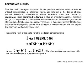
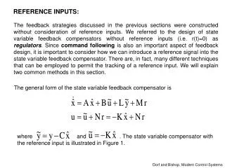
where and . The state variable compensator with the reference input is illustrated in Figure 1. REFERENCE INPUTS: The feedback strategies discussed in the previous sections were constructed without consideration of reference inputs. We referred to the design of state variable feedback compensators without reference inputs (i.e. r(t)=0) as regulators. Since command following is also an important aspect of feedback design, it is important to consider how we can introduce a reference signal into the state variable feedback compensator. There are, in fact, many different techniques that can be employed to permit the tracking of a reference input. We will explain two common methods in this section. The general form of the state variable feedback compensator is Dorf and Bishop, Modern Control Systems

System model u x C y r + N + Observer + Control Law -K - C Figure 1. State variable compensator with a reference input. Notice that when M=0 and N=0, the compensator reduces to the regulator described earlier.

The compensator’s key design parameters required to implement the command tracking of the reference input are M and N. When the reference input is a scalar signal (i.e., a single input), the parameter M is a column vector of length n, where n is the length of the state vector x, and N is a scalar. Here, we consider two possibilities for selecting M and N. In the first case, we select M and N so that the estimation error e(t) is independent of the reference input r(t). In the second case, we select M and N so that the tracking error y(t)-r(t) is utilized as an input to the compensator. These two cases will result in implementations wherein the compensator is in the feedback loop in the first case and in the forward loop in the second case. Employing the generalized compensator, the estimation error is found to be described by the differential equation or Dorf and Bishop, Modern Control Systems

Suppose that we select Then the corresponding estimation error is given by In this case, the estimation error is independent of the reference input r(t). This is the identical result found in th previous section, where we considered the observer design assuming no reference inputs. The remaining task is to determine a suitable value of N, since the value of M follows from the equation M=BN. For example, we might choose N to obtain a zero steady-state tracking error to a step input r(t). With M=BN, we find that the compensator is given by

System model r + y u N + Observer Control Law -K Compensator Figure 2. State variable compensator with a reference input and M=BN. Dorf and Bishop, Modern Control Systems

As an alternative approach, suppose that we select N=0 and M=-L. Then, the compensator is given by which can be written as In this formulation, the observer is driven by the tracking error y-r. The reference input tracking implementation is illustrated in Figure 3.

System model Control Law Compensator Observer -K y u r + - Figure 3. State variable compensator with a reference input and N=0and M=-L. Notice that in the first implementation (with M=BN) the compensator is in the feedback loop, whereas in the second implementation (N=0 and M=-L) the compensator is in the forward path. These two implementations are representative of possibilities open to control system designers when considering reference inputs. Dorf and Bishop, Modern Control Systems

Example: Consider the system given in state variable form where In the Simulink model, we will utilize full-state feedback, which means that the entire state vector (x1 and x2) is available for feedback. Therefore the output is y=x. where Dorf and Bishop, Modern Control Systems

The full-state feedback control law is where r is a reference input.

x1 x1 x2 In this example, we use a sine wave as the reference input. We can choose different input forms. The feedback gain matrix is chosen as This choice places the closed-loop poles (that is, the eigenvalues of A-BK) at s1=-1 and s2=-3. Using Simulink allows us easy access to the feedback gain matrix so that simulation studies using varying feedback gain sets can be readily performed. In the simulation presented here, the initial consitions are chosen to be x1(0)=1 and x2(0)=0.

SCALING THE REFERENCE INPUT: For good tracking performance we want Consider the performance issue in the frequency domanin. Use the final value theorem MIT-Open Course Notes

Thus, for good performance, we want Example: Consider the system The closed loop poles can be located at s=-5 and s=-6 MIT-Open Course Notes

The transfer function is Assume that r(t) is a step, then by the final value theorem As seen from the result, our step response is quite poor! MIT-Open Course Notes

is the extra gain used to scale the closed-loop transfer function. One solution is to scale the reference input r(t) so that Now we have So that If we take , then So with a step input

We can compute Note that this development assumed that r was constant, but it could also be used if r is a slowly time-varying command. So the steady state step error is now zero, but is this OK?

clc;clear a=[1 1;1 2];b=[1 0]';c=[1 0];d=0; k=[14 57]; Nbar=-15; sys1=ss(a-b*k,b,c,d); sys2=ss(a-b*k,b*Nbar,c,d); t=[0:.025:4]; [y,t,x]=step(sys1,t); [y2,t2,x2]=step(sys2,t); plot(t,y,'--',t2,y2,'Linewidth',2);axis([0 4 -1 1.2]);grid; legend('u=r-Kx','u=Nbar*r-Kx','Location','SouthEast') xlabel('time (sec)');ylabel('Y output');title('Step Response') As seen from the response, there is a big improvement, but transient part is a bit weird. MIT-Open Course Notes

NONLINEAR SYSTEMS When engineers analyze and design nonlinear dynamical systems in electrical circuits, mechanical systems, control systems, and other engineering disciplines, they need to absorb and digest a wide range of nonlinear analysis tools. Most of the nonlinear systems can be modeled by a finite number of first-order ordinary differential equations. (1) Defining vectors

We can write equation (1) as follows (2) Equation (2) is the generalization of state-space respresentation to nonlinear systems. The vector x is called the state vector of the system, and the function u is the input. Similarly, the system output is obtained via the so-called read out equation. (3) Equation (2) and (3) are referred to as the state space realization of the nonlinear system. Special Cases: An important special case of equation (2) is when the input u is identically zero. In this case, the equation takes the form (4) This equation is referred to as the unforced state equation.

k(y) b m f(t) The second special case occurs when f(x,t) is not a function of time. In this case we can write (5) in which case the system is said to be autonomous. Autonomous systems are invariant to shifts in the time origin in the sense that changing the time variable from t to τ=t-α does not change the right-hand side of the state equation. In this example, we consider the more realistic case of hardening spring in which the force strengthens as y increases. We can approximate this model by taking y Marquez JH, Nonlinear Control Systems

With this constant, the differential equation results in the following: (6) Defining state variables x1=y, x2=dy/dt results in the following state space realization which is the form In particular, if u=0, then Marquez JH, Nonlinear Control Systems

Equilibrium Points (Singular points): An important concept when dealing with the state equation is that of equilibrium point. Definition 1.1 A point x=xe in the state space is said to be an equilibrium point of the autonomous system if it has the property that whenever the state of the system starts at xe, it remains at xe for all future time. According to this definition, the equilibrium points of (4) are the real roots of the equation f(xe)=0. This is clear from equation (4). Indeed, if it follows that xe is constant and, by definition, it is an equilibrium point.

Example: Consider the following first-order system • where r is a paremeter. To find the equilibrium pointsof the system, we solve the equation r+x2=0 and we obtain • If r<0, the system has two equilibrium points, namely x=±r0.5. • If r=0, both of the equilibrium points in (i) collapse into one and the same, and the unique equilibrium point is x=0 • Finally, if r>0, then the system has no equilibrium points.

x(0)=0.5 x(0)=0.5

x(0)=-0.4

Example: Consider the following nonlinear second-order system At t=0 x(0)=1, dx(0)/dt=2

Phase Plane Initial values (1,2) x Convergent solution

Phase Plane (3,6) x Divergent solution.

At state of equilibrium dx1/dt=x2=0 The system has two singular points, one at (0,0) and the other at (-3,0) x1=0 x1=-3 =0

(-3.01,0) (0.1,0) The motion patterns of the system trajectories in the vicinity of the two singular points have different natures. The trajectories move towards the point x=0 while moving away from the point x=-3. Stable Unstable One may wonder why an equilibrium point of a second-order system is called a singular point. To anser this, let us examine the slope of the trajectories. The slope of the phase trajectory passing through a point (x1,x2) is determined by Slotine and Weiping, Applied Nonlinear Control.

With the functions f1 and f2 assumed to be single valued, there is usually a definite value for the slope at any given point in phase plane. This implies that the phase trajectories will not intersect. At singular points, however, the value of the slope is 0/0, i.e., the slope is indeterminate. Many trajectories may intersect at such points. The indeterminancy of the slope accounts for the adjective “singular”. Singular points are very important features in phase plane. Examination of the singular points can reveal a great deal of information about the properties of a system. In fact, stability of linear systems in uniquely characterized by the nature of their singular points. For nonlinear systems, besides singular points, there may be more complex features, such as limit cycles. Figure 4. Phase portrait of the nonlinear system. Slotine and Weiping, Applied Nonlinear Control.

Dorf and Bishop, Modern Control Systems